Week 9

Sociology 106: Quantitative Sociological Methods

March 17, 2026

Agenda

Housekeeping:

  • Annotated bibliography & Spring Recess

Statistical content — three parts:

  • Part 1: Hypothesis testing — the logic
  • Part 2: t-tests for means and group differences (+ proportion z-test)
  • Part 3: Chi-squared test — associations between two categorical variables

In-class lab:

  • Example of how to apply hypothesis tests to your research data

Housekeeping

Annotated Bibliography

  • Due Thursday, March 19
  • Happy to answer last-minute questions after class!
  • Example on bCourses under the Research Paper folder

Weekly Assignment #8

  • Due Thursday, April 2 (after Spring Recess)
  • Involves applying today’s hypothesis testing tools to your research dataset

Spring Recess

  • March 24 — enjoy the break!
  • Use that time to relax and work on your paper proposal with outline due on 4/16

Where We Are in the Course

  • Week 7: sampling distributions and the Central Limit Theorem
  • Week 8: confidence intervals — estimating population parameters from samples
  • This week (Week 9): hypothesis testing + tests for associations
  • Weeks 10–13: regression analysis (OLS and logistic)

Main idea: Last week we built confidence intervals — a range of plausible values for a parameter. Today we flip the question: given a specific claim about the population, how likely are our sample results if that claim were true?

The chain of inference so far:

Week 7: Population → Sample → Statistic → Sampling distribution

Week 8: Sample → Statistic → Confidence interval → Inference

Week 9: Null hypothesis + Sample statistic → Test statistic → p-value → Decision

Last Week: Recap

Concept Key idea Example
Point estimate Best single guess for population parameter \(\hat{p} = 0.449\) (GSS env. support)
Standard error How uncertain is the estimate? \(SE(\hat{p}) = 0.015\)
Confidence interval Range likely to contain the true parameter 95% CI: [0.420, 0.478]
z vs t Proportions → z; Means → t \(z^* = 1.96\); \(t^* = 2.447\) (\(df = 6\))

Connection to today:

Last week we estimated unknown population parameters and surrounded them with intervals. Today we start from a specific claim about the population — and ask whether our data are consistent with it.

Questions?

Part 1: Hypothesis Testing

Can we rule out chance as an explanation?

What Is a Hypothesis Test?

A hypothesis test is a formal statistical procedure for evaluating whether a finding is likely due to chance.

The core steps:

  1. State a null hypothesis (\(H_0\)): “there is no real effect” — the finding is just chance
  2. Choose a tail: does theory predict a direction? → one-tailed; otherwise → two-tailed (default)
  3. Compute a test statistic: how far is our sample result from what \(H_0\) would predict?
  4. Calculate a p-value: if \(H_0\) is true, how likely is a result this extreme?
  5. Decide: if the p-value is small enough, reject \(H_0\); accept \(H_1\)

The core logic:

We don’t prove the null hypothesis wrong — we ask: if it were true, how surprising would our data be? If very surprising, we have grounds to doubt the null.

A Motivating Example: James Bond

James Bond claims he can tell whether a martini is shaken or stirred just by tasting it.

The experiment: Give him 16 randomly prepared martinis. He correctly identifies 13 out of 16.

Null hypothesis (\(H_0\)): He’s just guessing — each trial is a 50-50 coin flip (\(\pi = 0.5\))

Alternative hypothesis (\(H_1\)): He can genuinely tell the difference — he performs better than random guessing (\(\pi > 0.5\))

The question: If he were just guessing, how likely is it that he’d get 13 or more right out of 16?

# P(X >= 13) under H0: X ~ Binomial(n = 16, p = 0.5)
1 - pbinom(12, size = 16, prob = 0.5)
[1] 0.01063538

Probability ≈ 1.1% — very unlikely if he were just guessing. We have strong evidence he can actually tell the difference.

P-values

A p-value is the probability of observing a test statistic as extreme as (or more extreme than) the one we got, assuming the null hypothesis is true

  • James Bond: \(p = 0.011\) — if guessing randomly, only 1.1% chance of ≥ 13/16 correct

Critical misconception:

What the p-value is NOT: the probability that \(H_0\) is true. The null hypothesis is either true or false — it doesn’t have a probability.

What the p-value is : P(data this extreme | \(H_0\) true) — the probability of observing results at least this extreme, assuming the null holds. It answers: “if the null were true, how often would we see data like ours?” — not “how likely is the null to be true?”

p-value Interpretation
Very small (e.g., 0.001) Data would be very surprising under \(H_0\) → strong evidence against \(H_0\)
Small (e.g., 0.03) Data somewhat unlikely under \(H_0\) → moderate evidence against \(H_0\)
Large (e.g., 0.40) Data consistent with \(H_0\) → no reason to doubt \(H_0\)
  • ❌ The probability that \(H_0\) is true
  • ❌ The probability that we made an error
  • ❌ How large or important the effect is
  • ❌ Whether the finding matters in practice

Statistical ≠ substantive significance:

A result can be statistically significant (\(p < 0.05\)) but substantively trivial — the effect is real but tiny. With large samples, even meaningless effects can reach significance. Always report the size of the effect, not just whether it is significant.

Significance Levels

How small does the p-value need to be before we reject \(H_0\)?

We set a significance level \(\alpha\) in advance — the threshold below which we’ll reject:

  • Most common: \(\alpha = 0.05\) — we use this in this class
  • Sometimes people use: \(\alpha = 0.01\), \(\alpha = 0.10\)

Decision rule:

Result Decision
\(p < \alpha\) Reject \(H_0\) — accept \(H_1\); say the result is “statistically significant”
\(p \geq \alpha\) Fail to reject \(H_0\) — we do not “accept” \(H_0\), we just lack evidence to reject it

Why “fail to reject” — not “accept”?

A negative result doesn’t prove the null is true. A small sample may simply be too underpowered to detect a real effect. We might be failing to reject because the effect doesn’t exist — or because we didn’t have enough data to see it.

Two Ways to Be Wrong

Every decision has two possible mistakes:

\(H_0\) is True \(H_0\) is False
Reject \(H_0\) Type I error (false positive) Correct ✓
Fail to reject \(H_0\) Correct ✓ Type II error (false negative)


In plain language: the paramedic

You arrive at an accident. Is the victim alive (\(H_0\)) or dead (\(H_1\))?

  • Type I error: You declare them dead when they’re alive → they don’t get treatment. Catastrophic.
  • Type II error: You rush a dead person to hospital. Wasteful, but not deadly.

Here you’d want a very small \(\alpha\) — the cost of the errors is not symmetric.

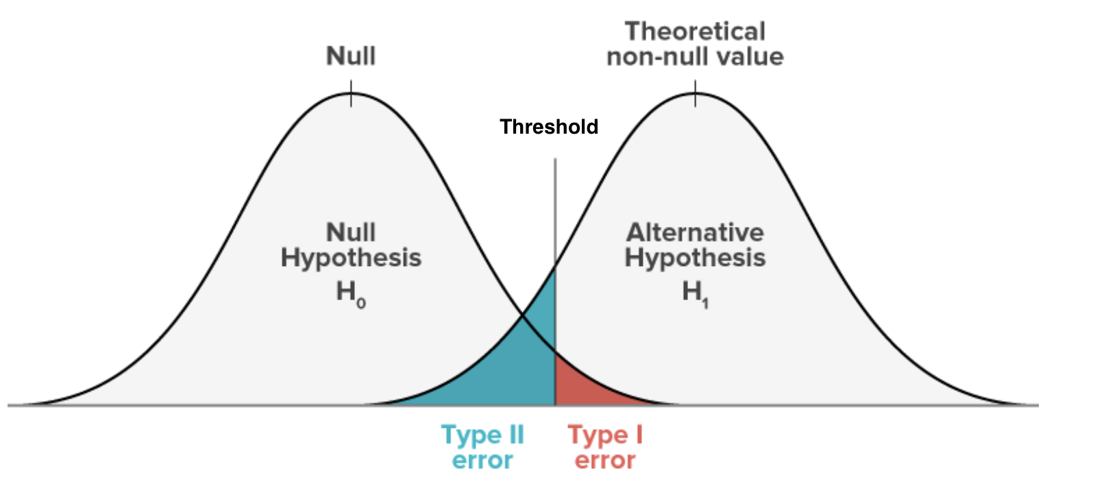
Trade-off between Type I and II Error

Note

The trade-off: Moving the threshold right reduces Type I error but increases Type II error — and vice versa. You can shrink both by increasing \(n\), which pulls the two distributions apart.

  • Lower \(\alpha\) (e.g., 0.05 vs 0.10) → less Type I risk, more Type II risk
  • Larger \(N\) → distributions pull apart → less Type II risk without increasing Type I risk

One- and Two-Tailed Tests

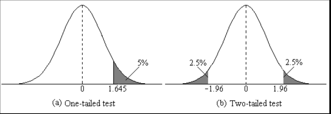
A one-tailed test checks for a significant effect in one specific direction

  • \(H_0: \pi \leq 0.50\) vs. \(H_1: \pi > 0.50\)
  • All of \(\alpha\) is in one tail — critical value is lower — and therefore easier to reject \(H_0\), but only if the effect is in the predicted direction

James Bond (one-tailed): Did he perform better than random guessing?

# P(X >= 13): all probability in upper tail
1 - pbinom(12, size = 16, prob = 0.5)
[1] 0.01063538

A two-tailed test checks for a significant effect in either direction

  • \(H_0: \pi = 0.50\) vs. \(H_1: \pi \neq 0.50\)
  • \(\alpha\) is split equally — 2.5% in each tail — critical value is higher ; more conservative and more common in social science

James Bond (two-tailed): Did he perform differently from random guessing?
# Multiply by 2: account for both tails
2 * (1 - pbinom(12, size = 16, prob = 0.5))
[1] 0.02127075

One-tailed (top) vs. two-tailed (bottom) tests
  • One-tailed: rejection region entirely on one side
  • Two-tailed: rejection region split — requires a more extreme result to reject
Scenario Recommended
Theory strongly predicts the direction One-tailed (use sparingly!)
No strong directional prediction Two-tailed (default)

Default to two-tailed:

Unless you have a strong, pre-specified theoretical reason to predict direction, use a two-tailed test. Effects in the “unexpected” direction are often theoretically important!

CIs and Hypothesis Tests

Last week’s confidence intervals and today’s hypothesis tests are two sides of the same coin:

  • If the 95% CI does not contain the null value \(\mu_0\)reject \(H_0\) at \(\alpha = 0.05\)
  • If the 95% CI contains the null value → fail to reject \(H_0\)
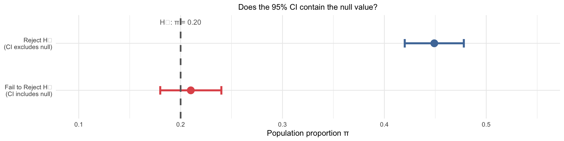
The equivalence:

The 95% CI is precisely the set of null values you would fail to reject at \(\alpha = 0.05\). Testing and estimation are equivalent — they just frame the same question differently.

Questions?

Part 2: t-Tests for Means and Group Differences

Testing associations involving a continuous outcome variable

Three Common Tests

Test When to use Key statistic Example
One-sample t-test Comparing sample to population; \(\bar{x} = \mu\) t-score Do Berkeley students work more than 20 hrs/week on average?
Two-sample t-test Comparing means of two groups; \(\bar{x_1} = \bar{x_2}\) t-score Do men and women differ in hours worked per week?
Proportion test Testing proportions; test if \(\hat{p} = P\) z-score Is union membership among women different from 20%?

All three tests follow the same steps:

  1. state \(H_0\)
  2. choose one- or two-tailed
  3. compute a test statistic measuring how far the sample result is from \(H_0\)
  4. find the p-value under the null distribution
  5. decide

Test 1: One-Sample t-Test for a Mean

Compare the sample to the population.

General form of the one-sample t-test:

\[H_0: \mu = \mu_0 \qquad \text{(sample mean equals a specified population value)}\]

\(H_1\) depends on whether the research hypothesis predicts a direction:

Alternative Test type When to use
\(H_1: \mu \neq \mu_0\) Two-tailed No predicted direction — default choice
\(H_1: \mu > \mu_0\) One-tailed (upper) Theory predicts sample is higher than \(\mu_0\)
\(H_1: \mu < \mu_0\) One-tailed (lower) Theory predicts sample is lower than \(\mu_0\)

Running example: Is the mean hours worked per week by U.S. adults equal to 40 hours?

  • \(H_0: \mu = 40\) — the population mean is 40 hours
  • \(H_1: \mu \neq 40\) — the population mean is something other than 40 (two-tailed)
  • Significance level: \(\alpha = 0.05\)

Under \(H_0\), the test statistic follows a t-distribution with \(df = n - 1\):

\[t = \frac{\bar{x} - \mu_0}{s / \sqrt{n}}\]

Step What to compute Formula/Rule
1 State \(H_0\) and \(H_1\) \(H_0: \mu = \mu_0\); choose \(H_1\) based on theory
2 One- or two-tailed? Does theory predict a direction? → one-tailed; otherwise → two-tailed (default)
3 Sample mean & SE \(\bar{x}\); \(SE = s / \sqrt{n}\)
4 t-statistic \(t = (\bar{x} - \mu_0) / SE\)
5 p-value See below

Step 2 determines the p-value formula:

  • Two-tailed (\(H_1: \mu \neq \mu_0\)): 2 * pt(-abs(t), df = n - 1)
  • One-tailed upper (\(H_1: \mu > \mu_0\)): 1 - pt(t, df = n - 1)
  • One-tailed lower (\(H_1: \mu < \mu_0\)): pt(t, df = n - 1)

mu = 40 sets the null hypothesis value — R tests whether the true population mean equals 40.

hrs_clean <- attain |> filter(!is.na(hrs1))

t1_result <- t.test(hrs_clean$hrs1, mu = 40)
t1_result

    One Sample t-test

data:  hrs_clean$hrs1
t = 5.0511, df = 1899, p-value = 0.0000004813
alternative hypothesis: true mean is not equal to 40
95 percent confidence interval:
 41.01450 42.30234
sample estimates:
mean of x 
 41.65842 

Reading the t.test() output:

  • t = 5.05: our sample mean (41.66 hrs) is 5.05 standard errors above the null value of 40 — that is a large distance
  • df = 1899: degrees of freedom (\(n - 1\)); we have a large sample
  • p-value < 0.001: if the true mean were exactly 40 hrs, a result this extreme would occur less than 0.1% of the time — very strong evidence against \(H_0\)
  • 95% CI [41.01, 42.3]: we are 95% confident the true mean is between 41.01 and 42.3 hrs — this range does not include 40, confirming we reject \(H_0\)
  • mean of x = 41.66: sample mean hours worked per week

The sample mean hours worked per week was 41.66 hours. A one-sample t-test showed this is significantly different from 40 hours (\(p\) < 0.001). We reject \(H_0\); we accept \(H_1\): U.S. adults in this sample work significantly more than a standard 40-hour week.

The 95% CI [41.01, 42.3] does not contain 40 — this is the CI equivalent of rejecting \(H_0\) at \(\alpha = 0.05\).

Test 2: Two-Sample t-Test

Running example: Do union members work a different number of hours per week than non-members?

  • \(H_0\): \(\mu_{\text{union}} = \mu_{\text{non-union}}\) (equivalently: \(\mu_1 - \mu_2 = 0\))
  • \(H_1\): \(\mu_{\text{union}} \neq \mu_{\text{non-union}}\)

Under \(H_0\), the test statistic:

\[t = \frac{\bar{x}_1 - \bar{x}_2}{SE_{\text{diff}}} \quad \text{where} \quad SE_{\text{diff}} = \sqrt{\frac{s_1^2}{n_1} + \frac{s_2^2}{n_2}}\]

Degrees of freedom: \(df \approx n_1 + n_2 - 2\) (R uses Welch’s correction, adjusting df when variances differ)

union_hrs    <- attain |>
  filter(union_member == 1, !is.na(hrs1)) |> pull(hrs1)
nonunion_hrs <- attain |>
  filter(union_member == 0, !is.na(hrs1), !is.na(union)) |> pull(hrs1)

t2_result <- t.test(union_hrs, nonunion_hrs)
t2_result

    Welch Two Sample t-test

data:  union_hrs and nonunion_hrs
t = 1.8535, df = 316.26, p-value = 0.06475
alternative hypothesis: true difference in means is not equal to 0
95 percent confidence interval:
 -0.1122722  3.7619461
sample estimates:
mean of x mean of y 
 43.52284  41.69801 

Reading the t.test() output:

  • t = 1.85: the observed difference in means (43.52 − 41.7 = 1.82 hrs) is 1.85 standard errors from zero
  • df = 316.3: Welch’s adjusted degrees of freedom (R accounts for unequal variances)
  • p-value = 0.065: a difference this large would occur 6.5% of the time by chance if \(H_0\) were true — does not clear \(\alpha = 0.05\)
  • 95% CI [-0.11, 3.76]: plausible range for the true difference \(\mu_{\text{union}} - \mu_{\text{non-union}}\) — this interval contains 0, consistent with failing to reject \(H_0\)
  • means: union = 43.52 hrs, non-union = 41.7 hrs

Union members worked an average of 43.52 hours per week, compared to 41.7 hours for non-members (difference = 1.82 hrs). A two-sample t-test showed this difference was not statistically significant (\(p\) = 0.065). We fail to reject \(H_0\): we cannot conclude union members work different hours than non-members.

The 95% CI on the difference [-0.11, 3.76] includes 0 — consistent with failing to reject \(H_0\) at \(\alpha = 0.05\).

Test 3: Testing a Proportion

We follow the same set up, but use a slightly different distribution.

Running example: Is the proportion of U.S. adults who are union members equal to 20%?

  • \(H_0: \pi = 0.20\)
  • \(H_1: \pi \neq 0.20\) (two-tailed)
  • Significance level: \(\alpha = 0.05\)

Under \(H_0\), the sampling distribution of \(\hat{p}\) is approximately:

\[\hat{p} \sim N\!\left(\pi_0,\; SE_0\right) \quad \text{where} \quad SE_0 = \sqrt{\frac{\pi_0(1-\pi_0)}{n}}\]

Key distinction — testing vs. estimation:

When building a CI, use \(SE = \sqrt{\hat{p}(1-\hat{p})/n}\) (the sample estimate). When testing a hypothesis, use \(SE_0 = \sqrt{\pi_0(1-\pi_0)/n}\) (the null value).

Step 1: Compute the standard error under \(H_0\):

\[SE_0 = \sqrt{\frac{\pi_0(1-\pi_0)}{n}} = \sqrt{\frac{0.20 \times 0.80}{n}}\]

Step 2: Compute the z-statistic:

\[z = \frac{\hat{p} - \pi_0}{SE_0}\]

Step 3: Calculate the p-value:

Test R code
Two-tailed 2 * pnorm(-abs(z))
One-tailed (upper) pnorm(-abs(z))

prop.test() handles the SE and test statistic automatically — just supply the count of successes, the sample size, and the null value.

n <- sum(!is.na(attain$union))
x <- sum(attain$union_member, na.rm = TRUE)   # number of union members

# prop.test(successes, n, p = null_value, correct = FALSE)
t3_result <- prop.test(x, n, p = 0.20, correct = FALSE)
t3_result

    1-sample proportions test without continuity correction

data:  x out of n, null probability 0.2
X-squared = 62.306, df = 1, p-value = 0.000000000000002941
alternative hypothesis: true p is not equal to 0.2
95 percent confidence interval:
 0.1150532 0.1445757
sample estimates:
        p 
0.1290973 

Reading the prop.test() output:

  • X-squared = 62.31: the test statistic (\(z^2\)); our sample proportion is 7.89 standard errors from the null value of 0.20
  • p-value = 0: if the true proportion were exactly 20%, a result this far away would occur 0% of the time — this is our evidence against \(H_0\)
  • 95% CI [0.115, 0.145]: plausible range for the true union membership rate — check whether this contains 0.20
  • p = 0.129: our sample union membership rate (\(\hat{p}\))

Note: correct = FALSE turns off the continuity correction — appropriate when \(n\) is large.

The sample union membership rate was 0.129 (12.9%). A proportion test showed this was significantly different from 20% (\(p\) = 0). We reject \(H_0\); we accept \(H_1\).

The 95% CI [0.115, 0.145] does not contain 0.20 — the null value falls entirely outside the plausible range for the true proportion, confirming we reject \(H_0\).

Worked Example: Household Income

Using the GSS attain dataset, we test whether respondents’ mean household income differs from the U.S. national median household income of $30,000 (1991 Census benchmark, the year these data were collected).

The income91 variable records household income as midpoints of GSS income brackets (e.g., $500, $2,000 … $100,000).

Research question: Does mean household income in the GSS sample differ from the national median?

Question: Write the hypothesis notation and specify whether this is a one- or two-tailed test.

Null hypothesis: Mean household income in the sample equals the national median:

\[H_0: \mu = \$30{,}000\]

Alternative hypothesis: Mean household income is different from the national median:

\[H_1: \mu \neq \$30{,}000\]

Two-tailed — the research question asks whether income differs, not specifically whether it is higher or lower.

The logic:

We have no directional prediction going in — the GSS sample could plausibly earn more or less than the national median. So we split the rejection region (\(\alpha = 5\%\)) equally across both tails (2.5% each). This is the more conservative and more common choice in social science.

inc_clean <- attain |> filter(!is.na(income91))

we_result <- t.test(inc_clean$income91, mu = 30000)
we_result

    One Sample t-test

data:  inc_clean$income91
t = 14.205, df = 2635, p-value < 0.00000000000000022
alternative hypothesis: true mean is not equal to 30000
95 percent confidence interval:
 36547.93 38645.17
sample estimates:
mean of x 
 37596.55 
cat("p-value =", format.pval(we_result$p.value), "\n")
p-value = < 0.000000000000000222 

Since t.test() runs a two-tailed test by default, the p-value already reflects both tails.

Since \(p < 0.001 < \alpha = 0.05\), we reject \(H_0\); we accept \(H_1\).

Conclusion:

The mean household income in our sample ($37,597)) is significantly higher than the national median of $30,000 (\(p\) < 0.001). The 95% CI [$36,548, $38,645] does not contain $30,000, confirming we reject \(H_0\). GSS respondents earn more than the national median, and this gap is unlikely to be due to sampling error alone.

Questions?

Part 3: The Chi-Squared Test

Testing associations between two categorical variables

The Family of Hypothesis Tests

Every test we’ve covered this week asks the same fundamental question: is there a relationship between variables? The choice of test depends entirely on the types of variables involved.

What we’re testing Outcome variable Grouping variable Method
Is a proportion = \(P\)? Binary z-test
Is a mean = \(\mu_0\)? Continuous one-sample t-test
Do two group means differ? Continuous Binary (2 groups) two-sample t-test
Do 3+ group means differ? Continuous Categorical (3+ groups) ANOVA (not covered)
Are two categorical variables independent? Categorical Categorical chi-squared test

The key decision:

Is your outcome variable continuous? → use a t-test (or ANOVA for 3+ groups). Is your outcome variable categorical? → use chi-squared. Note: chi-squared works for any number of categories — not just binary variables.

t-Tests vs. Chi-Squared: Parallel Logic

Both tests ask “Is \(X\) related to \(Y\)?” — for different variable combinations:

Question: Does the mean of a continuous outcome differ across groups?

  • Outcome: continuous (e.g., hours worked)
  • Group: binary/categorical (e.g., union membership)
  • \(H_0\): \(\mu_{\text{union}} = \mu_{\text{non-union}}\)
  • Test stat: \(t = (\bar{x}_1 - \bar{x}_2) / SE_{\text{diff}}\), compared to t-distribution

Our example: Do union members work a different number of hours than non-members? Focusing on the difference in means between the two groups.

Question: Does the distribution of a categorical outcome differ across groups?

  • Outcome: categorical (e.g., union membership — yes/no)
  • Group: categorical (e.g., sex)
  • \(H_0\): Union membership and sex are independent
  • Test stat: \(\chi^2 = \sum (n_{ij} - \hat{n}_{ij})^2 / \hat{n}_{ij}\), compared to \(\chi^2\) distribution

Our example: Is union membership associated with sex?

Two-sample t-test Chi-squared
\(H_0\) \(\mu_1 = \mu_2\) \(X\) and \(Y\) are independent
Outcome type Continuous Categorical
Group type Binary/categorical Categorical
Test statistic \(t\) \(\chi^2\)
Distribution t (\(df = n_1+n_2-2\)) \(\chi^2\) (\(df = (I{-}1)(J{-}1)\))
Measure of effect Difference in means Difference in proportions
In R t.test(x, y) chisq.test(table)

Choosing your test for hw8:

Does your research question compare a continuous outcome across groups? → two-sample t-test. Does it compare the rates of a categorical outcome across groups? → chi-squared.

Review: Contingency Tables

A contingency table shows the joint distribution of two categorical variables — counts of observations in each combination of categories

Non-member Union member Total
Female \(n_{11}\) \(n_{12}\) \(n_{1\bullet}\)
Male \(n_{21}\) \(n_{22}\) \(n_{2\bullet}\)
Total \(n_{\bullet 1}\) \(n_{\bullet 2}\) \(n\)
attain_ct <- attain |>
  filter(!is.na(union), !is.na(sex)) |>
  mutate(union_lab = if_else(union_member == 1, "Union", "Non-member"))

# Count table with row and column totals
tab <- table(attain_ct$sex, attain_ct$union_lab)
addmargins(tab)
        
         Non-member Union  Sum
  female       1003   105 1108
  male          724   151  875
  Sum          1727   256 1983
# Row proportions: union membership rate within each sex
round(prop.table(tab, margin = 1), 3)
        
         Non-member Union
  female      0.905 0.095
  male        0.827 0.173

The Chi-Squared Logic

The null hypothesis: The two categorical variables are independent — knowing someone’s category on one variable tells us nothing about their category on the other

\[H_0: \text{no association between } X \text{ and } Y\]

Under independence, the expected count in each cell:

\[\hat{n}_{ij} = \frac{(\text{row total}_i) \times (\text{column total}_j)}{n}\]

This is what the table would look like if the two variables had no relationship at all.

The test asks: Are the observed cell counts far enough from the expected cell counts that we doubt independence?

The Chi-Squared Test Statistic

\[\chi^2 = \sum_{i}\sum_{j} \frac{(n_{ij} - \hat{n}_{ij})^2}{\hat{n}_{ij}}\]

where \(n_{ij}\) = observed and \(\hat{n}_{ij}\) = expected count in cell \((i, j)\)

  • Large \(\chi^2\): observed counts are far from expected → evidence against independence
  • Small \(\chi^2\): observed counts are close to expected → consistent with independence
  • Degrees of freedom: \((I-1)(J-1)\), where \(I\) = number of rows, \(J\) = number of columns

Assumptions:

  1. Data are a random sample from the population
  2. Expected count in each cell ≥ 5 — if not, the chi-squared approximation may not be reliable

Worked Example 1: Sex and Union Membership

Research question: Is there a significant association between sex and union membership?

attain_ct |>
  count(sex, union_lab) |>
  pivot_wider(names_from = union_lab, values_from = n) |>
  mutate(Total = `Non-member` + Union)
# A tibble: 2 × 4
  sex    `Non-member` Union Total
  <chr>         <int> <int> <int>
1 female         1003   105  1108
2 male            724   151   875
tab <- table(attain_ct$sex, attain_ct$union_lab)

# Row proportions: union rate within each sex
round(prop.table(tab, margin = 1), 3)
        
         Non-member Union
  female      0.905 0.095
  male        0.827 0.173
chisq_result <- chisq.test(tab, correct = FALSE)
round(chisq_result$expected, 1)  # verify all expected counts ≥ 5
        
         Non-member Union
  female        965   143
  male          762   113
chisq_result

    Pearson's Chi-squared test

data:  tab
X-squared = 26.325, df = 1, p-value = 0.0000002886

correct = FALSE turns off Yates’ continuity correction — standard when all expected counts ≥ 5

Men were 7.8 percentage points more likely to be union members than women (17.3% vs. 9.5%). A chi-squared test showed this association was statistically significant (\(\chi^2\)(1) = 26.3, \(p\) < 0.001). We reject \(H_0\); we accept \(H_1\): sex and union membership are not independent in this sample.

Important:

Chi-squared only tells you whether an association exists — not its direction or magnitude. Always supplement with a difference in proportions.

Worked Example 2: Sex and Educational Attainment

\(H_0\): Sex and college attainment are independent. \(H_1\): They are not. \(\alpha = 0.05\).

attain_deg <- attain |>
  filter(!is.na(sex), !is.na(degree)) |>
  mutate(college = if_else(degree %in% c("bachelor", "graduate"), "College+", "No college"))

attain_deg |>
  count(sex, college) |>
  pivot_wider(names_from = college, values_from = n) |>
  mutate(Total = `College+` + `No college`)
# A tibble: 2 × 4
  sex    `College+` `No college` Total
  <chr>       <int>        <int> <int>
1 female        382         1316  1698
2 male          331          953  1284
tab2 <- table(attain_deg$sex, attain_deg$college)
round(chisq.test(tab2, correct = FALSE)$expected, 1)  # verify ≥ 5
        
         College+ No college
  female      406       1292
  male        307        977
chisq.test(tab2, correct = FALSE)

    Pearson's Chi-squared test

data:  tab2
X-squared = 4.3281, df = 1, p-value = 0.03749
attain_deg |>
  count(sex, college) |>
  group_by(sex) |>
  mutate(prop = round(n / sum(n), 3)) |>
  select(-n) |>
  pivot_wider(names_from = college, values_from = prop)
# A tibble: 2 × 3
# Groups:   sex [2]
  sex    `College+` `No college`
  <chr>       <dbl>        <dbl>
1 female      0.225        0.775
2 male        0.258        0.742
college_props <- attain_deg |>
  count(sex, college) |>
  group_by(sex) |>
  mutate(prop = n / sum(n)) |>
  filter(college == "College+")

cat("Difference in proportions:", round(college_props$prop[1] - college_props$prop[2], 3), "\n")
Difference in proportions: -0.033 

Women were 3.3 percentage points less likely than men to have a college degree (22.5% vs. 25.8%). A chi-squared test showed this association was statistically significant (\(\chi^2\)(1) = 4.3, \(p\) = 0.038). We reject \(H_0\); we accept \(H_1\): sex and college attainment are not independent in this sample.

Writing up chi-squared results — always include:

  1. The group rates — which group is higher and by how much?
  2. The test result\(\chi^2\)(df), \(p\)-value
  3. The decision — reject \(H_0\); accept \(H_1\) / fail to reject \(H_0\)
  4. Plain-language conclusion tied to the research question

Questions?

Key Takeaways

  • A hypothesis test asks: if the null were true, how likely is our data?
  • The p-value is the probability of seeing a result this extreme if the null were true — NOT the probability the null is true
  • Reject the null when p < 0.05; otherwise fail to reject (never “accept” the null)
  • Default to two-tailed; use one-tailed only when theory predicts a specific direction

Connection to Week 8:

If the 95% CI does not contain the null value → reject the null at 0.05. Tests and CIs are two sides of the same coin.

Test Use when R function Example
One-sample t-test Is the mean = some value? t.test(x, mu = value) Do GSS respondents earn differently from $30,000?
Two-sample t-test Do two group means differ? t.test(x, y) Do union members work more hours than non-members?
Proportion test Is a proportion = some value? prop.test(x, n, p = value) Is union membership different from 20%?
Chi-squared Are two categorical variables independent? chisq.test(table) Is union membership associated with sex?

Always report: the group statistic(s), the p-value, your decision, and a plain-language conclusion.

  • Tests whether two categorical variables are independent
  • Compares the counts you observed to what you’d expect if there were no relationship
  • All expected counts must be ≥ 5
  • Only tells you whether an association exists — not direction or strength
  • Always supplement with a difference in proportions

Why This Matters for the Rest of the Course

  • Weeks 10–13 (Regression): OLS is essentially the two-sample t-test extended to multiple variables simultaneously. Every regression coefficient comes with its own t-test and p-value — built on exactly the same logic we used today.
  • Your research paper: You will almost certainly use regression. But the interpretation of \(p\)-values, test statistics, and significance thresholds is identical to what we covered today.

Key takeaway:

Hypothesis testing is not just a tool for this week — it is the core inferential logic running through all of statistics. Every result in your paper will be evaluated with the same p-value framework we built today.

Questions?