Week 5

Sociology 106: Quantitative Sociological Methods

February 17, 2026

Housekeeping

HW #1: Great job everyone ! Lots of great coding

HW #2: Really great job finding data, asking questions, and responding to prompts. Make sure to check rendering and answer all of the questions.

HW #3: due Thursday, February 19 at 11:59 PM

Paper Proposal (5%): due Thursday, February 26, 11:59 PM

• A two-page double-spaced proposal for your final paper.
• Here’s an example of what I expect.

Academic Integrity Asignment due Friday, May 8, 11:59 PM

Questions?

Course Overview

Where we’ve been: Finding data and describing it (graphs, summary statistics)

Where we’re going: Inferring things about the “real world” from data

This week: We step back from actual data to think about the processes that generated the data — probability models that will power our inferences

Agenda

Basics of Probability

• Probability models
• Sample spaces
• Density curves
• Rules of probability
• Probabilities of multiple events

Probability Models

To make inferences, we first need to model the processes that generate data

Randomness and Probability

A phenomenon is random if individual outcomes are uncertain but there is a regular distribution of outcomes over many repetitions

• Examples: rolling a die, playing the lottery, a coin toss

The probability of an outcome is the proportion of times it would occur in a very large number of independent repetitions

\[P(A) = \frac{\text{number of repetitions where A occurs}}{\text{total number of repetitions}}\]

Repetitions are independent if the result of one does not influence the result of others

Example: A Coin Toss

While the result of any single coin toss is random, the result over many tosses is predictable as long as the tosses are independent

If tosses are independent, then we can say that the probability of tossing “heads” is the proportion of “heads” in a large number of trials

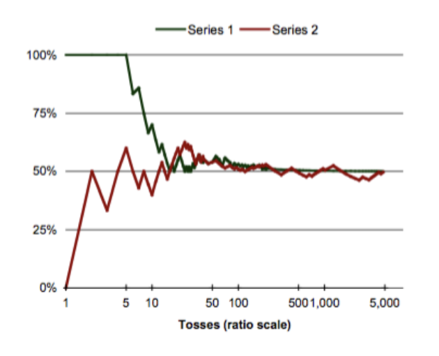
This illustrates how randomness at the individual level produces predictability at the aggregate level

Calculating Probabilities

Empirical approach

• We can calculate probabilities by observing many trials of a random phenomenon

• Then calclute the probability¹ by taking a sample proportion of the number of times the outcome occurred

Theoretical approach

• We can also calculate theoretical probabilities based on assumptions about the random phenomena (i.e., all die rolls equally likely)

1. This is an estimate that improves as we observe more trials

Probability Models

Probability models are theoretical models that mathematically describe the outcome of random processes. They consist of two parts:

1. Sample space (S): the set of all possible outcomes of a random process
   • Ex: Sample space for a six-sided die is 1, 2, 3, 4, 5, 6
   • An event is a subset of the sample space (e.g., rollling an even number)
2. A probability for each possible event in the sample space S
   • Ex: rolling an even number 3/6 or 1/2

Properties of Probability Models

Three fundamental properties:

1. Range: Probabilities for any given event range from 0 (can’t happen) to 1 (happens every time)
   • Formally, for any event A: \(0 \leq P(A) \leq 1\)
   • So, the range of probability must be between 0 and 1

2. Exhaustiveness: \(P(S) = 1\). That is, the sample space is exhaustive of all possibilities

• In other words, there cannot be any limits on the probability of an occurance

3. Complement rule: The probability of an event not occurring is 1 minus the probability that it does occur:
   • \(P(\text{not } A) = 1 - P(A)\)
   • \(P(\text{not } A)\) is called the complement of A

Probability Models: Example

Probability model for a coin toss:

• Sample space S: {Heads, Tails}

• Probabilities (assuming a fair coin):

  • \(P(\text{Heads}) = 0.5\)
  • \(P(\text{Tails}) = 0.5\)

Check: Does this fit the properties?

1. Range: Both probabilities are between 0 and 1 ✓

2. Exhaustiveness: \(0.5 + 0.5 = 1\) ✓

3. Complement: \(P(\text{not Heads}) = P(\text{Tails}) = 1 - 0.5 = 0.5\) ✓

Sample Spaces

Every probability model starts by defining what outcomes are possible

Compound Events

Understanding sample space becomes most useful when we want to predict compound events that are the result of multiple trials

Calculate the probability of compound events by enumerating all possible outcomes and assigning a probability to each outcome

Example: What’s the probability of getting two heads in two coin flips?

We need to consider all possible outcomes and their probabilities

Example 1: Order matters

A basketball player shoots three free throws. Each shot is either a Hit (H) or Miss (M).

Sample space (all possible sequences):

\[S = \{HHH, HHM, HMH, HMM, MHH, MHM, MMH, MMM\}\]

• Total outcomes: 8
• Reason: Each shot has 2 outcomes → \(2^3 = 8\)
• 🔑 Order matters (HHM ≠ HMH)
  • HHM = Hit, Hit, Miss
  • HMH = Hit, Miss, Hit
  • These are different sequences!

Example 2: Order doesn’t matter

Now we only care about how many baskets are made, not the order

Sample space:

\[S = \{0, 1, 2, 3\}\]

• Each value represents the number of hits
• Total outcomes: 4
• 🔑 Order doesn’t matter
  • HMH and MHH both → 2 baskets
  • We collapse multiple sequences into single counts

Complement Shortcut: “At Least One”

The complement rule is especially useful for “at least one” problems

Example: What is the probability of getting at least one head in 3 coin flips?

We could list every outcome with at least one head… but it’s easier to use the complement:

\[P(\text{at least one head}) = 1 - P(\text{no heads})\]

\[= 1 - P(TTT) = 1 - \frac{1}{8} = \frac{7}{8}\]

Why this works: “at least one head” and “no heads” are complements — one of them must happen, so their probabilities sum to 1

Whenever you see “at least one,” think complement!

Example 3: Continuous outcomes

A nutrition researcher feeds a new diet to a lab rat and measures weight gain (grams)

Sample space:

\[S = [0, \infty)\]

• Any non-negative real number is possible
• Infinite number of outcomes
• 🔑 Continuous sample space
  • Can’t list all outcomes individually
  • Must use intervals and density curves

Back to the Two Coin Flips Example

Question: What’s the probability of getting two heads in two coin flips?

For two fair flips, the sample space is:

\[S = \{HH, HT, TH, TT\}\]

Each outcome is equally likely, so each has probability \(1/4\)

Let event \(A = \{\text{two heads}\} = \{HH\}\)

\[P(A) = P(HH) = \frac{1}{4}\]

Equivalent multiplication view (independent flips):

\[P(HH) = P(H)\times P(H) = \frac{1}{2}\times\frac{1}{2} = \frac{1}{4}\]

Discrete vs. Continuous Sample Spaces

Discrete sample spaces deal with data that can only take on certain values, known in advance (that is, categorical data)

• Example: Throwing a single die → \(S = \{1, 2, 3, 4, 5, 6\}\), each with probability \(1/6\)
• These are straightforward because we can list all possible outcomes

Continuous sample spaces contain an infinite number of outcomes. They are typically intervals of possible, continuously distributed outcomes

• Example: Picking a random real number between 0 and 1 → \(S = [0,1]\)

Question: How do we assign probabilities to outcomes in an infinite sample space?

Probabilities in Continuous Sample Spaces

We use density curves to represent probabilities across the continuous sample space, and compute probabilities for intervals as the area under the curve

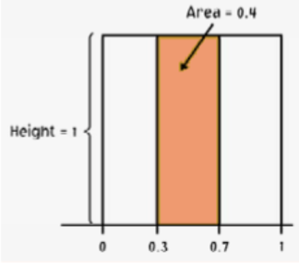
Example: Uniform density curve over \(S = [0,1]\) (all outcomes equally likely)

The shaded portion represents:

\(P(0.3 \leq x \leq 0.7) = (0.7 - 0.3) \times 1 = 0.4\)

Uniform density curve with shaded region between 0.3 and 0.7

Density Curves: Properties and Types

Properties:

• P(single point) = 0 — only intervals have non-zero probability
• Total area under the curve = 1
• Density curves are always non-negative

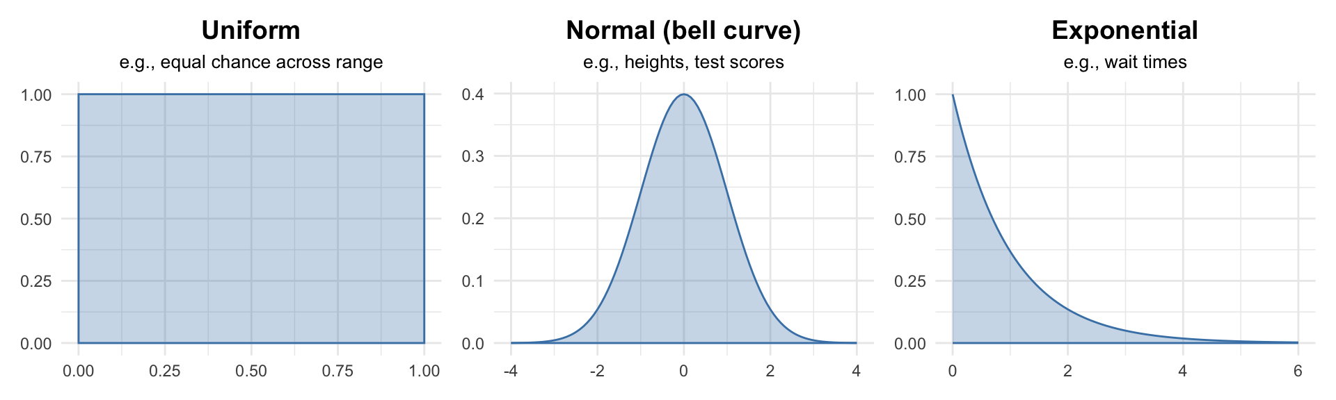
Common types we’ll encounter (we’ll use these extensively when we study the normal distribution):

Rules of Probability

Now that we know what outcomes are possible, we need rules for calculating the probability of combined events

• Use the Addition Rule when the question asks for “A or B”
• Use the Multiplication Rule when the question asks for “A and B”

Addition Rule: Union of “A or B”

The union of A and B (“A or B”) consists of outcomes that are in A, or in B, or in both A and B. Notation: \(A \cup B\)

• Use when question says “or”
• Special case: Disjoint events

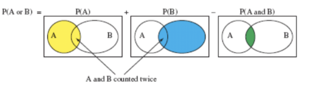
For the union of two events,

\[P(A \text{ or } B) = P(A) + P(B) - P(A \text{ and } B)\]

We subtract \(P(A \text{ and } B)\) to avoid double-counting outcomes in both events

Notice: even in an “or” problem, we still need the overlap term \(P(A \text{ and } B)\)

If the events are disjoint (mutually exclusive), then \(P(A \text{ and } B) = 0\)

\[P(A \text{ or } B) = P(A) + P(B)\]

Disjoint events have no overlap, so there’s nothing to subtract

Addition Rule: Worked Example

Example: I draw one card from a standard deck. What is the probability that I draw a club or a face card?

• \(P(\text{club}) = 13/52\) (13 clubs in the deck)
• \(P(\text{face card}) = 12/52\) (4 jacks + 4 queens + 4 kings)
• \(P(\text{club and face card}) = 3/52\) (jack, queen, king of clubs)

Applying the addition rule:

\[P(\text{club or face card}) = \frac{13}{52} + \frac{12}{52} - \frac{3}{52} = \frac{22}{52} \approx 0.42\]

We subtract \(3/52\) because the jack, queen, and king of clubs are both clubs and face cards — without subtracting, we’d count them twice!

Intersection and Conditional Probabilities

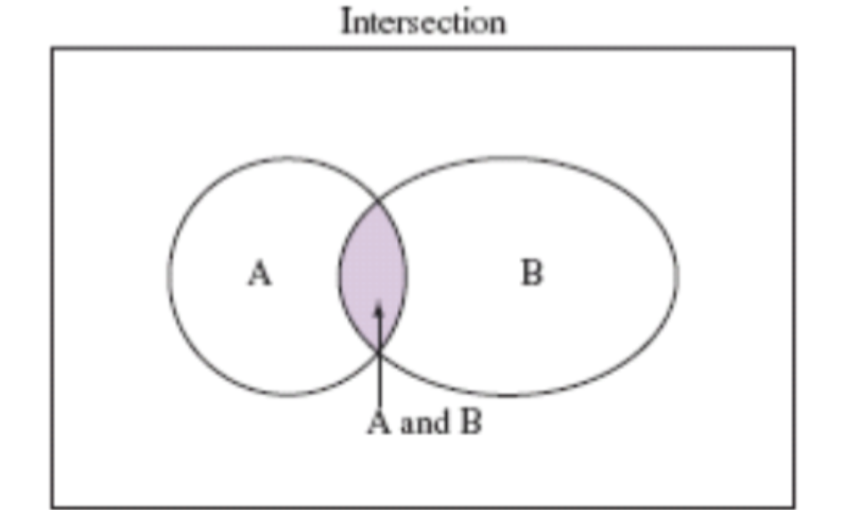
The intersection of A and B (\(A \cap B\)) consists of outcomes that are in both A and B — the overlap between two events

The conditional probability of event A, given that event B has occurred, is:

\[P(A|B) = \frac{P(A \text{ and } B)}{P(B)}\]

• \(P(A|B)\) is read as “the probability of A, given B”

Multiplication Rule: Intersection of “A and B”

Use this rule when the question asks for the probability that both events happen.

For the intersection of two events:

\[P(A \text{ and } B) = P(A) \times P(B|A)\]

Alternatively: \(P(A \text{ and } B) = P(B) \times P(A|B)\)

It doesn’t matter which event we choose first!

Independent Events

If two events are independent, the probability that one event occurs is not affected by whether the other event occurs

This implies:

• \(P(B|A) = P(B)\)
• \(P(A|B) = P(A)\)
• \(P(A \text{ and } B) = P(A) \times P(B)\)

Example: Coin flips are independent - knowing the first flip doesn’t tell you anything about the second flip

Independence and Sampling

A common way to determine independence: how are you sampling?

• With replacement: Put the item back before drawing again → draws are independent (probabilities don’t change)
• Without replacement: Keep the item out → draws are dependent (probabilities change after each draw)

Example: An urn has 7 red and 3 blue marbles

• With replacement: \(P(\text{Red 2nd draw}) = 7/10\) regardless of 1st draw
• Without replacement: \(P(\text{Red 2nd} | \text{Red 1st}) = 6/9\), but \(P(\text{Red 2nd} | \text{Blue 1st}) = 7/9\)

Multiplication Rule: Worked Example

Example: An urn has 7 red and 3 blue marbles

With replacement (independent draws):

\[P(RR) = P(R) \times P(R) = \frac{7}{10} \times \frac{7}{10} = \frac{49}{100}\]

Without replacement (dependent draws):

\[P(RR) = P(R_1) \times P(R_2 | R_1) = \frac{7}{10} \times \frac{6}{9} = \frac{42}{90}\]

Notice the difference: without replacement, getting a red marble first changes the probability of getting a red marble second

Questions?

Next Week: Probability Distributions

We will learn about random variables, which are numerical measurements of a random phenomenon that take on particular values (or ranges of values) with certain probabilities

• We can represent any variable we’ve talked about so far in this class—hair color of students, height, income—as a random variable

Then, we’ll look at probability models of the distributions of random variables

Weekly Assignment #4

You’ll answer some questions based on lecture today. You will not need a dataset.

HW #4: due Thursday, February 26 at 11:59 PM

Paper Proposal (5%)

A two-page double-spaced proposal for your final paper is due on bCourses by Thursday, February 26 at 11:59 PM. Here’s an example.

Your proposal should include:

1. Research question - What are you trying to answer?
2. Why it matters - Why should we care about this question?
3. Hypotheses - What do you think the answer is, and why?
4. Data source - What dataset will you use?
5. Key variables - Identify your independent and dependent variables

Note: You do not need to discuss statistical techniques at this point.