Week 4

Sociology 106: Quantitative Sociological Methods

February 10, 2026

Housekeeping

HW #1: due tonight (Tuesday, February 10) by 11:59 PM – Extended deadline - any questions?

HW #2: due Thursday, February 12, 11:59 PM - Ideal to use your final project data

Paper Proposal (5%): due Thursday, February 26, 11:59 PM - A two-page double-spaced proposal for your final paper. - Here’s an example of what I expect.

Academic Integrity Asignment due Friday, May 8, 11:59 PM

Questions?

Agenda

Summarizing distributions:

Relative and marginal frequencies
Measures of the central tendency
- Mean, median, and mode
Measures of dispersion
- Percentiles and standard deviation / variance
Association between two variables
- Comparing proportions: difference in proportions, relative risk ratio
- Comparing distributions: covariance and correlation

What is a good research question?

Specifies a relationship between two or more variables
- Not just “What is X?” but “How does X relate to Y?”
Is answerable with data — can be investigated empirically
Has sociological significance — connects to broader theory or social patterns
Is clearly scoped — specific enough to study, not so narrow it’s trivial

Examples from sociology:

“Is there an association between educational attainment and income in the U.S.?”
“Do marriage rates differ across racial groups, and how has this changed over time?”
“Is religious affiliation associated with political ideology?”

A good research question guides everything else: your data, your variables, and your choice of summary statistics or measures of association.

Frequencies

Frequencies: relative frequencies

Relative frequency (aka proportion): the frequency of observations for a given variable, divided by the total number of observations.

This is similar to a probability, though statisticians generally talk about probabilities existing “in the world” and relative frequencies existing “within the data”

Notation:

$p_{X=i} = \frac{n_{X=i}}{n_{total}}$
Sometimes $p_{X=i}$ is shortened to $p_i$

Relative frequency in the case of two variables:

$p_{X=i,Y=j} = \frac{n_{X=i,Y=j}}{n_{total}}$

Frequencies: marginal frequencies

The marginal (or conditional) proportion is the relative frequency of observations taking a certain value for a given variable (i.e., X), conditional on the observations taking a certain value for another variable (i.e., Y)

Notation:

$p_{X=i \mid Y=j} = \frac{n_{X=i,\,Y=j}}{n_{Y=j}}$
Sometimes $p_{X=i|Y=j}$ is shortened to $p_{ij}$

Frequencies: Examples

The table below is reconstructed from a published study:

	18th Century	19th Century
Publishing Trade	109	21
Other Occupations	53	82
Total	162	103

18th Century (marginal freq)
19th Century (marginal freq)
Relative freq

Marginal frequency of magazine founders’ occupations being in the publishing trade, conditional on the magazine being founded in the 18th century:

\[109/162 = 67.3\%\]

Marginal frequency of magazine founders’ occupations being in the publishing trade, conditional on the magazine being founded in the 19th century:

\[21/103 = 20.3\%\]

We can also recover the overall relative frequency from the same table — the number of all founders in the publishing trades, divided by all foundings:

\[(109 + 21)/(162 + 103) = 130/265 = 49.1\%\]

Frequencies: when to use

Relative frequencies are more useful if both variables are categorical, not continuous

If the variable is continuous, there may not be very many observations that have a certain value for a given variable
Example: yearly earnings (in dollars)—it would not be very informative to find the relative frequency of individuals with yearly earnings of $27,475

Same for marginal frequencies: more useful if both variables are categorical, not continuous

Frequencies: calculating in R

Now, let’s use R to calculate relative and marginal frequencies

Relative freq
Marginal freq (one group)
Marginal freq (two groups)

Relative frequency formula : $p_{X=i} = \frac{n_{X=i}}{n_{total}}$

attain |> 
  # count absolute frequencies
  count(marital) |> 
  # create a proportion
  mutate(proportion = n / sum(n))

# A tibble: 6 × 3
  marital      n proportion
  <chr>    <int>      <dbl>
1 divorced   446   0.149   
2 married   1541   0.515   
3 never ma   614   0.205   
4 separate   102   0.0341  
5 widowed    288   0.0963  
6 <NA>         1   0.000334

Marginal frequency for males. Formula : $p_{X=i \mid Y=j} = \frac{n_{X=i,\,Y=j}}{n_{Y=j}}$

attain |> 
  # Table of absolute freq for var1, 
  # for given value for var2
  filter(sex == "male") |> 
  count(marital) |> 
  # Use that table to create relative freq
  mutate(proportion = n / sum(n))

# A tibble: 5 × 3
  marital      n proportion
  <chr>    <int>      <dbl>
1 divorced   165     0.128 
2 married    730     0.566 
3 never ma   312     0.242 
4 separate    34     0.0264
5 widowed     49     0.0380

Marginal frequencies for both male and female. Formula : $p_{X=i \mid Y=j} = \frac{n_{X=i,\,Y=j}}{n_{Y=j}}$

attain |> 
  group_by(sex, marital) |> 
  summarize(n = n(), .groups = "drop_last") |> 
  mutate(proportion = n / sum(n))

# A tibble: 11 × 4
# Groups:   sex [2]
   sex    marital      n proportion
   <chr>  <chr>    <int>      <dbl>
 1 female divorced   281   0.165   
 2 female married    811   0.476   
 3 female never ma   302   0.177   
 4 female separate    68   0.0400  
 5 female widowed    239   0.140   
 6 female <NA>         1   0.000588
 7 male   divorced   165   0.128   
 8 male   married    730   0.566   
 9 male   never ma   312   0.242   
10 male   separate    34   0.0264  
11 male   widowed     49   0.0380

Questions?

Central Tendency & Dispersion

Central tendency: definitions

Mode: the value of a variable that occurs most often in the data set

Median: the middle data value, if the data are ordered by increasing value

If there are an even number of observations, the median is the midpoint between the two middle values

(Arithmetic) mean (aka average): the sum of all values in the data set, divided by the number of observations in the data set

\[\bar{x} = \frac{1}{n}\sum_{i=1}^{n}x_i\]

Central tendency: worked example

Example data of number of people 10 members of a high school class sent text messages to on Monday: 5, 2, 10, 4, 3, 2, 6, 15, 3, 2

Mode
Median
Mean
Summary

The value that occurs most often:

5, 2, 10, 4, 3, 2, 6, 15, 3, 2 — 2 appears 3 times, more than any other value

Mode = 2

Order the data, then find the middle value(s):

(2, 2, 2, 3, 3, 4, 5, 6, 10, 15)

Two middle observations — find the midpoint: $(3 + 4)/2$ = 3.5

Median = 3.5

Sum all values and divide by $n$:

(5+2+10+4+3+2+6+15+3+2) / 10 = 5.2

Mean = 5.2

Measure	Value
Mode	2
Median	3.5
Mean	5.2

Notice that mode (2) < median (3.5) < mean (5.2) — this is a sign of right skew, produced by the outliers 10 and 15

Central tendency: skewness

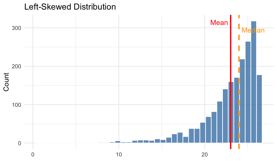
Relationship between mean, median, and mode tells us about the skew of a distribution:

Symmetric: Mean ≈ Median ≈ Mode.

Left-skewed
Right-skewed

Left-skewed (negative skew): the tail extends to the left. Mean < Median < Mode.

The mean is pulled toward the long left tail, so it is less than the median.

Right-skewed (positive skew): the tail extends to the right. Mean > Median > Mode.

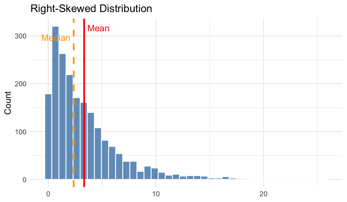
The mean is pulled toward the long right tail, so it is greater than the median.

Central tendency: summary

Mode can be used on variables of any level of measurement
- Less useful for continuous variables (e.g. yearly earnings)
- Generally the least useful; we usually prefer median or mean
Median cannot be used on nominal variables (requires ordering)
- Robust to outliers: median (3.5) does not depend on outliers 10 and 15
Mean cannot be used on nominal OR ordinal variables (requires meaningful distances)
- Takes into account the full distribution, but sensitive to outliers: mean (5.2) is pulled up by 10 and 15

Measurement	Mode	Median	Mean
Nominal	Yes	No	No
Ordinal	Yes	Yes	No
Continuous	Yes	Yes	Yes

Central tendency: calculating in R

These measures are simple to calculate in R. Let’s take a look:

Mean
Median
Mode

To calculate the mean respondent income in our sample, we can use the summarize() or summarise() function. Be sure to remove missing using na.rm = TRUE, which can affect the calculation.

# Mean
attain |> 
  summarise(mean = mean(rincom91, na.rm = TRUE)) |> 
  print()

# A tibble: 1 × 1
    mean
   <dbl>
1 25852.

We can do the same for the median using the median() function:

# Median
attain |> 
  summarise(median = median(rincom91, na.rm = TRUE)) |>
  print()

# A tibble: 1 × 1
  median
   <dbl>
1  21250

For the mode, we’ll simply want to count the number of obs (using count()) and take the largest number. We can do the following to see the most common marital status, which is unsurprisingly “married”.

attain |>
  count(marital) |>
  glimpse() |> 
  slice_max(n, n = 1, with_ties = FALSE) |>
  pull(marital)

Rows: 6
Columns: 2
$ marital <chr> "divorced", "married", "never ma", "separate", "widowed", NA
$ n       <int> 446, 1541, 614, 102, 288, 1

[1] "married"

Questions?

Dispersion: overview

Percentiles: the $k$th percentile of the variable is the value that has the property that at least $k$ percent of the data are less than or equal to it
Deviation from the mean: the difference between a data value and the sample mean
Sample variance: the average squared deviations
Sample standard deviation: the square root of the sample variance

Dispersion: percentiles

Percentiles: the $k$th percentile of the variable is the value that has the property that at least k percent of the data are less than or equal to it

Calculating the $k$th percentile:

Order the data from smallest to largest: $(x_1, ..., x_n)$
Calculate the index $i = \frac{k \times n_{total}}{100}$
If index is a whole number, the percentile is an average of the ith and the ($i$+1)th values in the ordered data
If index is not a whole number, round up to whole number, and the percentile is the $i$th number

Dispersion: percentile example

Example: calculating the 30th and 45th percentile of: (5, 2, 10, 4, 3, 2, 6, 15, 3, 2)

Step 1 — Order the data: (2, 2, 2, 3, 3, 4, 5, 6, 10, 15)

30th percentile
45th percentile

Step 2 — Calculate the index: $30 \times 10/100 = 3$

Step 3 — Index is a whole number, so average the 3rd and 4th values:

\[(2 + 3)/2 = \mathbf{2.5}\]

Step 2 — Calculate the index: $45 \times 10/100 = 4.5$

Step 3 — Index is not a whole number, so round up to 5 and take the 5th value:

\[\mathbf{3}\]

Dispersion: variance and std. deviation

Deviation from the mean: for observation $i$, the deviation is $x_i - \bar{x}$

Sample variance: the average* squared deviations

\[s^2 = \frac{1}{n-1}\sum_{i=1}^{n}(x_i - \bar{x})^2\]

Sample standard deviation: the square root of the variance

\[s = \sqrt{\frac{1}{n-1}\sum_{i=1}^{n}(x_i - \bar{x})^2}\]

Note

These “averages” are divided by $n-1$, not $n$.

Dispersion: why square deviations?

Why do we square the deviations?

Ensures that the deviations will always be positive
- But, using the absolute value could do the same
Gives greater weight to outliers
- This has good and bad properties

Unsatisfying answer: most of the statistical tools we will learn in the rest of the course are based on the standard deviation and variance, and these are the most commonly used measures of dispersion

Dispersion: comparing measures

The tradeoff is similar to medians vs. means:

Percentiles: information at one point in the distribution, but robust to outliers
- Like the median, which is the 50th percentile
Variance / SD: uses the entire distribution, but sensitive to outliers

Statistic	Nominal	Ordinal	Continuous
Percentiles	No	Yes	Yes
Variance / SD	No	No	Yes

Dispersion: calculating in R

How do we use R to calculate measures of dispersion? Let’s look at various measures of dispersion of respondents’ income in our attain dataset.

Percentiles
Variance
Standard Deviation
All at once

This will return the values at those specific percentiles–25th, 50th, and 75th. So, a respondent with an income of $32,500 is in the 75th percentile of the sample.

# Percentiles
attain |>
  summarise(
    p25 = quantile(rincom91, 0.25, na.rm = TRUE),
    p50 = quantile(rincom91, 0.50, na.rm = TRUE),
    p75 = quantile(rincom91, 0.75, na.rm = TRUE)
  ) |> 
  glimpse()

Rows: 1
Columns: 3
$ p25 <dbl> 11250
$ p50 <dbl> 21250
$ p75 <dbl> 32500

This will return the measure of variance in our sample for this specific income variable.

# Variance
attain |>
  summarise(variance = var(rincom91, na.rm = TRUE)) |> 
  glimpse()

Rows: 1
Columns: 1
$ variance <dbl> 432600678

This will return the standard deviation (std_dev) of variance in our sample for this specific income variable.

# Standard deviation
attain |>
  summarise(std_dev = sd(rincom91, na.rm = TRUE)) |> 
  glimpse()

Rows: 1
Columns: 1
$ std_dev <dbl> 20799.05

we can calculate all of these measures simultaneously. We can also calculate sd manually if we’d like.

Here I use the gt package to make the table output a bit nicer. Check out the documentation!

# Verify sd equals sqrt(var)
attain |>
  summarise(
    variance = var(rincom91, na.rm = TRUE),
    std_dev  = sd(rincom91, na.rm = TRUE),
    sqrt_var = sqrt(var(rincom91, na.rm = TRUE))
  ) |> 
  # use `gt` for nicer table formatting!
  gt::gt()

variance	std_dev	sqrt_var
432600678	20799.05	20799.05

Questions?

Association

Association: comparing proportions

Difference in proportions

$p_{x_i | y_j} - p_{x_i | y_k}$

The difference in the proportion of $x_i$ between group $j$ and group $k$
Expressed in percentage points
Easy to use, but occasionally misleading

Relative risk ratio

$p_{x_i | y_j} / p_{x_i | y_k}$

Ratio of proportions across groups
Scales proportions against each other (generally less misleading)

Tip

There is a big difference between “percentage point increase” and “percent increase.”

Association: proportions example

	18th Century	19th Century
Publishing Trade	109	21
Other Occupations	53	82
Total	162	103

Difference in proportions
Relative risk ratios

Difference in proportions of a magazine founder being in the publishing trade (x) in the 18th as compared to the 19th century (y):

\[109/162 - 21/103 = 67.3\% - 20.3\% = 47 \text{ percentage points}\]

This is an absolute difference—it tells you the raw gap between the two proportions.

“67.3% of 18th century founders were in publishing compared to 20.3% in the 19th century—a difference of 47 percentage points.”

Relative risk ratio of a magazine founder being in the publishing trade (x) in the 18th as compared to the 19th century (y):

\[(109/162)/(21/103) = 67.3\%/20.3\% = 3.32\]

This is a relative difference—how many times larger one proportion is than another.

“Magazine founders in the 18th century were 3.32 times as likely (or 232% more likely) to be in the publishing trade compared to those in the 19th century.”

Association: which measure to use?

Absolute difference (47 pp)

Better for practical/real-world impact.

Nearly 1/2 of 18th century founders were publishers vs. only 1/5 in the 19th century.

Relative risk (3.32x)

Better for the strength of the association.

18th century founders were over 3 times as likely to be a publisher.

Association: covariance

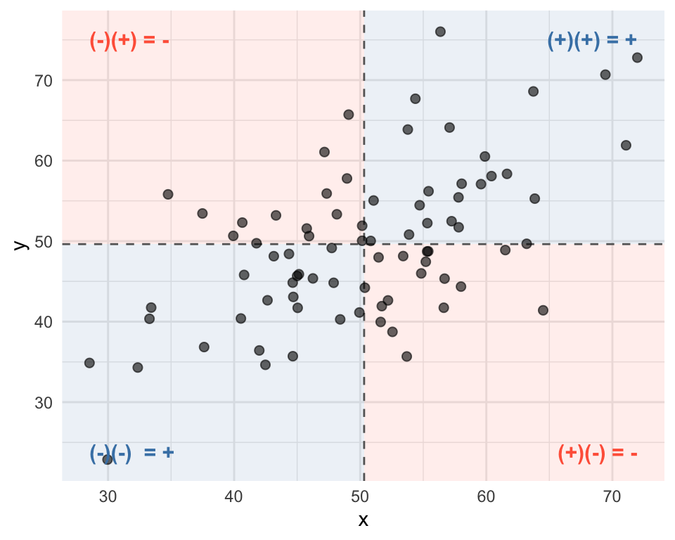
Covariance measures how two variables vary together. A positive means they move in the same direction; a negative means they move in opposite directions.

The covariance for $n$ observations on two variables $x$ and $y$ is equal to:

\[cov(x,y) = \frac{1}{n-1}\sum_{i=1}^{n}(x_i - \bar{x})(y_i - \bar{y})\]

The term $(x_i - \bar{x})(y_i - \bar{y})$ is:

Positive when $x_i$ and $y_i$ are both above or both below their means
Negative when one is above and the other below

Association: correlation

Correlation is a standardized measure of the linear association between two variables. Like covariance, it captures the direction of the relationship, but it also allows us to compare the strength across different variable pairs.

The correlation coefficient $r$ for $n$ observations on two variables x and y with sample standard deviations $s_x$ and $s_y$ is equal to:

\[r_{xy} = \frac{cov(x,y)}{s_x \times s_y}\]

Note

Covariance vs. correlation: Covariance tells you the direction of a relationship but its magnitude depends on the scale of the variables (dollars, years, etc.). Correlation standardizes covariance by dividing by the standard deviations, producing a unit-free measure that always falls between -1 and 1.

Association: correlation properties

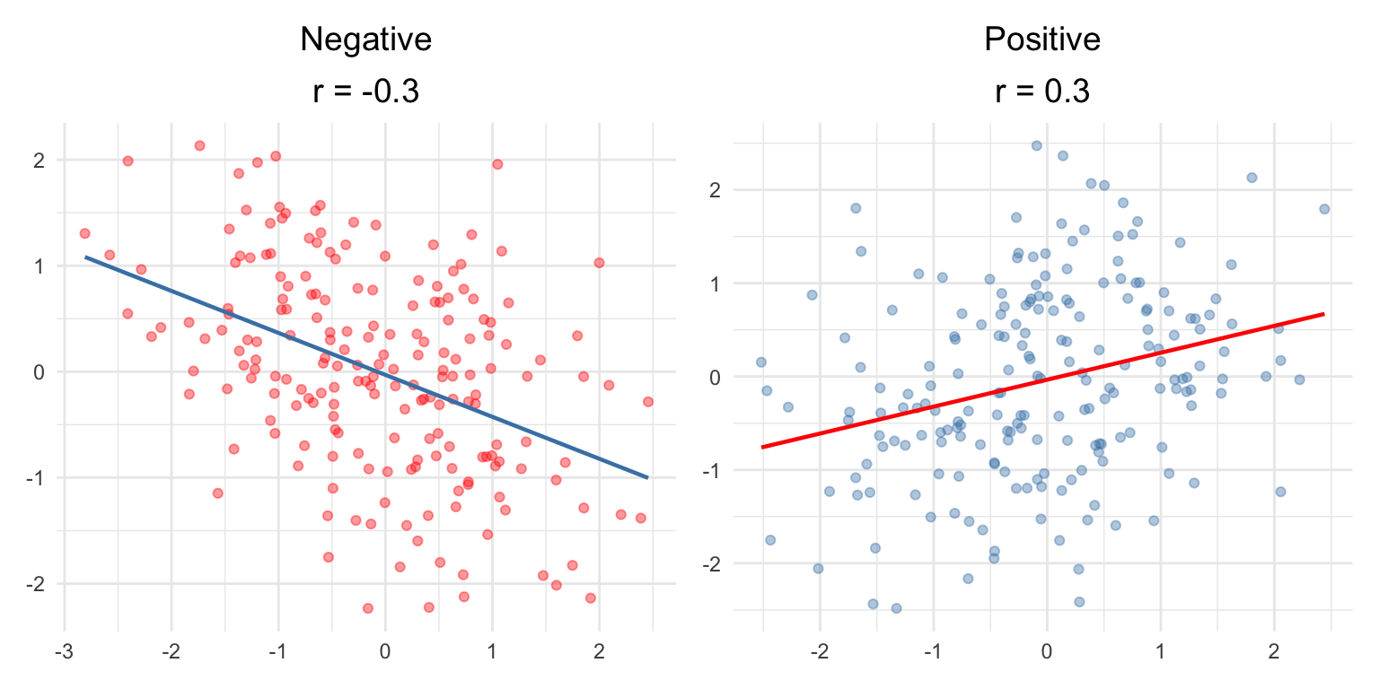
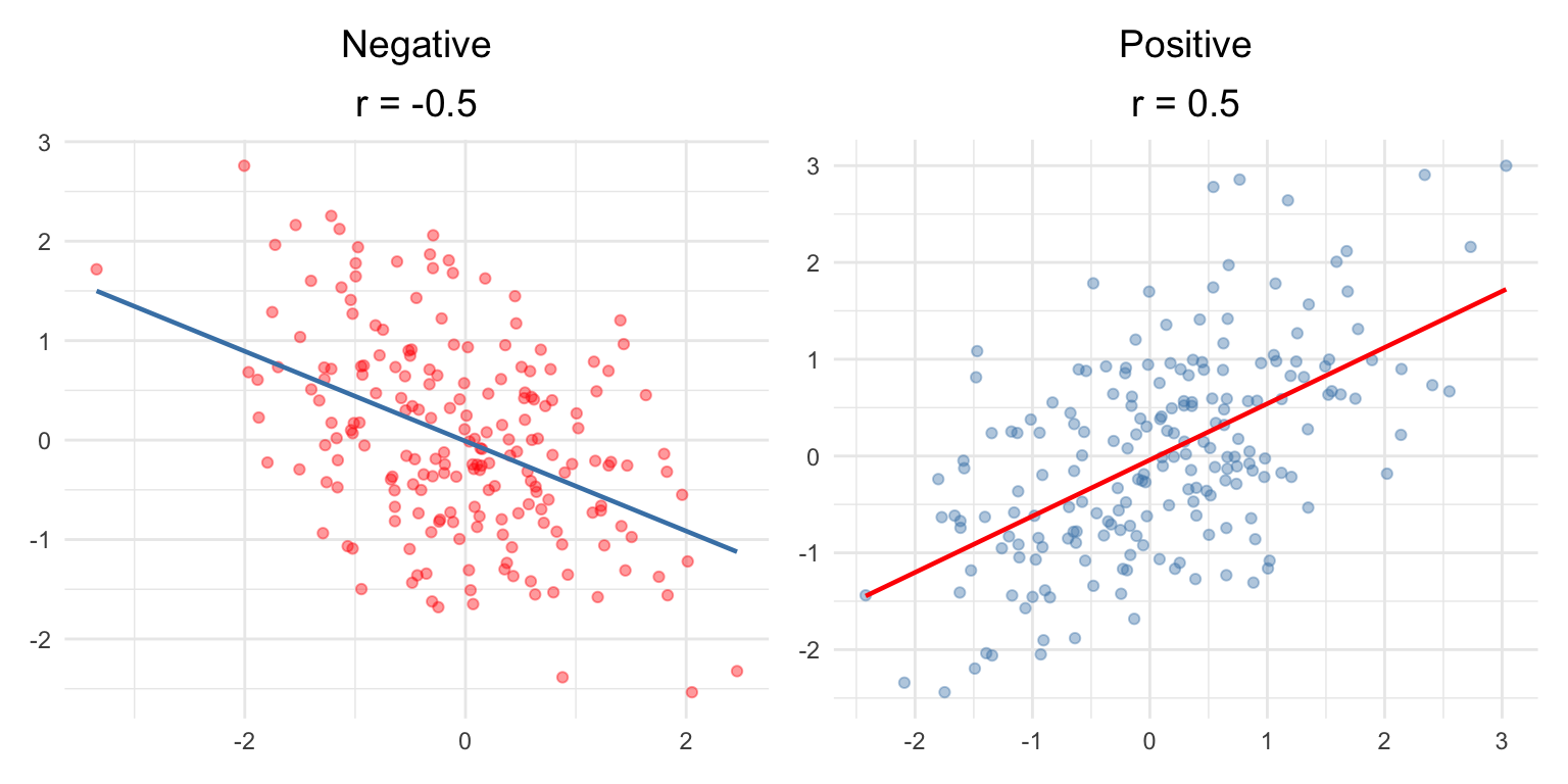
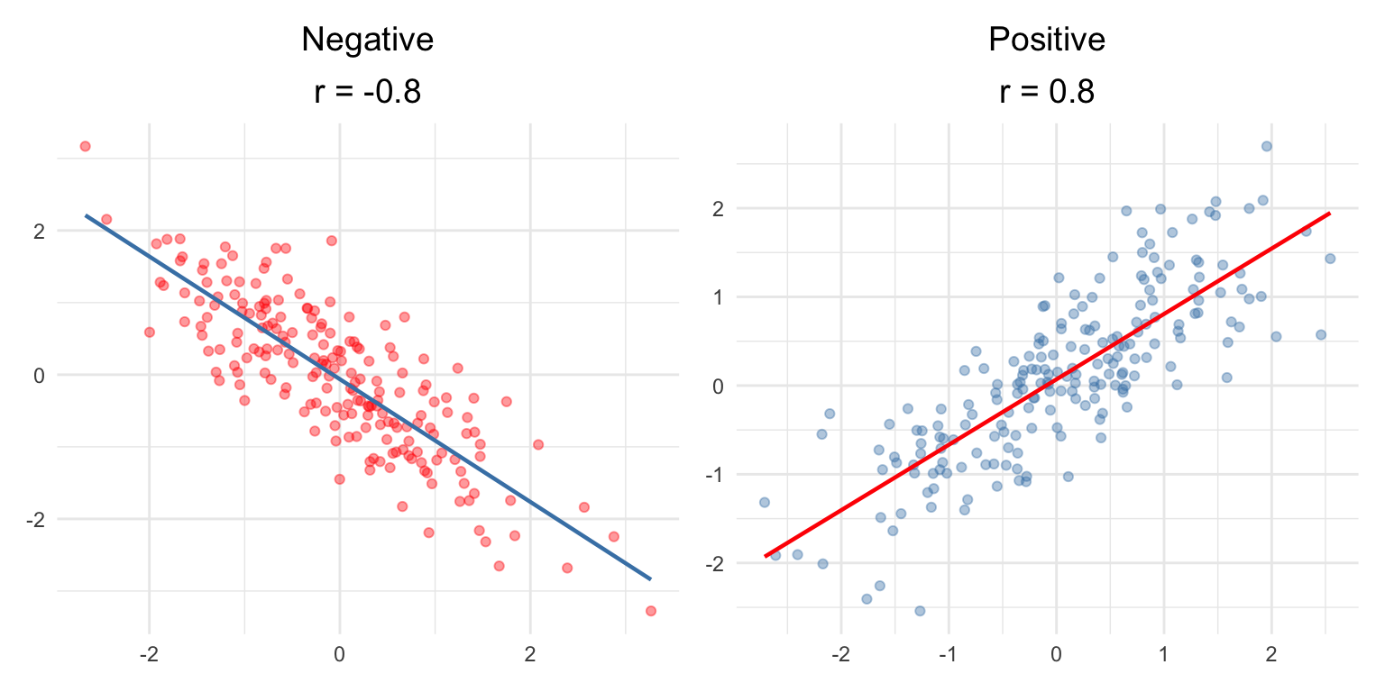
$r_{xy}$ is always between -1 and 1
$r_{xy}$ equals 1 if all observations fall along a straight line that has a positive slope (that is, as x increases, y increases in direct proportion)
$r_{xy}$ equals -1 if all observations fall along a straight line that has a negative slope (that is, as x increases, y decreases in direct proportion)
$r_{xy}$ does not depend on the scale of either $x$ and $y$

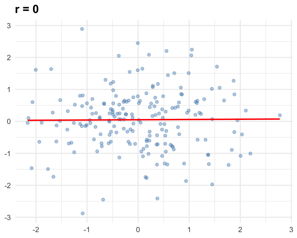
Weak: |r| = 0.10 to 0.39

Moderate: |r| = 0.40 to 0.69

Strong: |r| ≥ 0.70

Association: which measure for which data?

	Nominal	Ordinal	Continuous
Nominal	Difference in proportions; relative risk ratio	Difference in proportions; relative risk ratio	Difference in means between groups
Ordinal			Difference in means between groups
Continuous			Covariance, (Pearson’s) correlation coefficient

Association: calculating in R

Proportions
Covariance
Correlation

Step 1: Build marginal frequency tables

Let’s build a marginal freq table for bachelor’s degree and less than college

# Marginal freq for bachelor's degree holders
bach <- attain |>
  filter(degree == "bachelor", !is.na(marital)) |>
  count(marital) |>
  mutate(prop = n / sum(n))
bach

# A tibble: 5 × 3
  marital      n   prop
  <chr>    <int>  <dbl>
1 divorced    79 0.159 
2 married    287 0.579 
3 never ma   104 0.210 
4 separate     7 0.0141
5 widowed     19 0.0383

# Marginal freq for less than high school
lths <- attain |>
  filter(degree == "lt high", !is.na(marital)) |>
  count(marital) |>
  mutate(prop = n / sum(n))
lths

# A tibble: 5 × 3
  marital      n   prop
  <chr>    <int>  <dbl>
1 divorced    71 0.140 
2 married    212 0.418 
3 never ma    99 0.195 
4 separate    21 0.0414
5 widowed    104 0.205

Step 2: Difference in proportions (married)

Now let’s take the difference in those proportions of those that are married. How do we interpret this?

bach |> filter(marital == "married") |> pull(prop) -
  lths |> filter(marital == "married") |> pull(prop)

[1] 0.1604831

Click to reveal interpretation

58% of bachelor’s degree holders are married compared to 42% of those with less than a high school education—a difference of 16 percentage points.

Step 3: Relative risk ratio (married)

Finally let’s calculate the relative risk ratio of those that are married. How do we interpret this?

bach |> filter(marital == "married") |> pull(prop) /
  lths |> filter(marital == "married") |> pull(prop)

[1] 1.383797

Click to reveal interpretation

Bachelor’s degree holders are about 1.38 times as likely to be married compared to those with less than a high school education.

Let’s calulate the covariance of a respondent’s income and their household income. How do we interpret this?

# Covariance
attain |>
  summarize(covariance = cov(rincom91, income91, use = "complete.obs")) |>
  glimpse()

Rows: 1
Columns: 1
$ covariance <dbl> 376447249

Click to reveal interpretation

The positive covariance indicates that respondent income and household income tend to move in the same direction — when one is above its mean, the other tends to be as well. However, the magnitude (376,447,249) is hard to interpret on its own because it depends on the scale of both variables (dollars).

Now let’s calulate the correlation. How do we interpret this?

# Correlation coefficient
attain |>
  summarize(correlation = cor(rincom91, income91, use = "complete.obs"))

# A tibble: 1 × 1
  correlation
        <dbl>
1       0.671

Click to reveal interpretation

The correlation of 0.67 indicates a moderately strong, positive linear relationship between respondent income and household income. Unlike covariance, this value is standardized (between -1 and 1), making it easier to judge the strength of the association.

Questions?

Weekly Assignment #3

You’ll answer some questions based on lecture today. You will not need your own data for this but will use the attain data.

HW #3: due Thursday, February 19 at 11:59 PM

any questions?

In-class Lab

Let’s practice using the summary statistics we learned today:

Download lab2.qmd from bCourse under “assignments” > “Lab #2”
Place lab2.qmd in your labs folder. Your folder structure should now look like this:

soc106/
├── _quarto.yml
├── data/
│   └── attain.csv
├── assignments/
│   └── hw1.qmd
│   └── hw2.qmd
│   └── hw3.qmd
└── labs/
    └── lab1.qmd
    └── lab2.qmd

Use the Explorer button on the left to find and open lab2.qmd
Let’s work through it together!