Week 13

Sociology 106: Quantitative Sociological Methods

April 14, 2026

Agenda

Housekeeping:

HW #10, HW #11, Revised Proposal with Outline

Statistical content — two parts:

Part 1: Controlling for confounders — closing back doors in regression
Part 2: Interaction effects — when the relationship depends on context

Reading discussion:

Thompson & Keith (2001) — interactions in a classic race & gender study

In-class lab:

Running interactions on your research data

Housekeeping

Weekly Assignment #10

Due Thursday, April 16
Logistic regression on a binary outcome — covered last week

Weekly Assignment #11

Due Thursday, April 23
Run an interaction analysis on your research data (see Assignments slide)

Revised Proposal with Outline

Due Thursday, April 16 — two days away!
Describe whether your analysis will include any controls or interaction terms

In-class presentations

April 28/May 5 — 7–10 minutes per student, use this slide template to keep it short

Where We Are in the Course

Week 11: OLS regression — how strong is the linear relationship between X and Y?
Week 12: Logistic regression — predicting binary outcomes
This week (Week 13): Extensions — controlling for confounders and interaction effects
Next week (Week 14): More extensions — mediation and wrap-up

The big picture: from association to causal story

Weeks 11–12 asked: “Is there a relationship between X and Y?” This week asks: “Is that relationship spurious? And does it work the same way for everyone — or does it depend on who you are?” These questions bring us closer to causal inference and to understanding the social mechanisms behind the patterns we observe.

Questions?

Part 1: Controls and Confounding

Closing the back door

Why We Add Control Variables

We want to estimate the “causal” effect of X on Y. Three conditions for causality:

Condition	What it means
1. Correlation	X and Y are statistically associated
2. Temporal priority	X comes before Y in time
3. Non-spuriousness	No third variable Z is creating a false association between X and Y

A confounding variable Z:

Has a causal effect on X (Z → X)
Has a causal effect on Y (Z → Y)
Comes before both X and Y in time
Creates a spurious statistical association between X and Y

We remove the confound by controlling for Z in the regression: lm(Y ~ X + Z)

What “controlling for Z” actually means

Adding Z to the regression asks: “Among people with the same value of Z, what is the relationship between X and Y?” We are comparing like to like.

This is the foundation — but causal inference is harder

What we’re doing here is the workhorse strategy for observational causal inference. But it has real limits: we can only control for variables we actually observe and measure. Unmeasured confounders still bias our estimates — and we can never fully rule them out with regression alone.

Modern methods designed for this problem include: difference-in-differences (exploiting before/after comparisons), regression discontinuity (exploiting thresholds), and instrumental variable analysis (finding exogenous variation in X). This course builds the logic; but there are more sophisticated methods you’ll need to go deeper. For now: controlling for observed confounders is good practice, but “I controlled for everything” is always a theoretical claim, not a statistical guarantee.

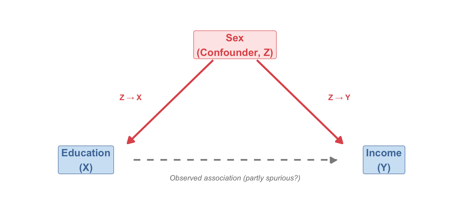
Confounding: The Path Model

Without controlling for Z, we observe a statistical association between X and Y. But that association is partly due to Z’s effects on both — not just the direct X → Y path.

Our running example:

X = Years of education
Y = Income (1991)
Z = Sex (a potential confounder)

Men and women may differ in both education level (Z → X) and in income (Z → Y). If we don’t control for sex, part of what looks like an “education effect” is really a “sex effect.”

A Classic Example: Computers and Test Scores

The Setup
The Resolution
What to Control For

In the early 1990s, researchers found: households with home computers had children with higher math test scores.

Does computer ownership cause better academic performance?

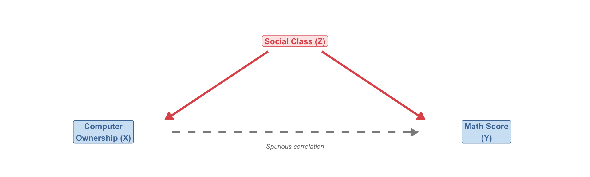
Social class caused both computer ownership and math achievement — it was the confound:

Higher-class families could afford computers (Z → X)
Higher-class families also provided better academic resources (Z → Y)

When researchers controlled for social class — comparing families at the same class level — the computer–test score correlation vanished.

The general lesson:

A variable Z is a confounder if: (1) Z → X, (2) Z → Y, and (3) Z precedes both X and Y in time. To remove its influence, we add Z to the regression: lm(Y ~ X + Z). Once we do this, we estimate the effect of X within levels of Z — comparing like with like.

A critical warning: not everything should be controlled

Only control for variables that: 1. Come before X and Y in time (prior common causes) 2. Are not themselves caused by X (otherwise you create new bias)

Do NOT control for:

Mediators (variables on the X → Y causal path) — this would underestimate X’s total effect
Colliders (variables caused by both X and Y) — this actually introduces new bias

For now: include controls that have a plausible prior causal connection to both your X and Y. We’ll cover mediation — and why you shouldn’t control for it — in Week 14.

# Bivariate: education → income
model_biv     <- lm(income91 ~ educ,               data = attain_sub)

# Control for sex
model_control <- lm(income91 ~ educ + sex_f,       data = attain_sub)

# Control for sex + age
model_multi   <- lm(income91 ~ educ + sex_f + age, data = attain_sub)

Adding variables with + holds each one constant while estimating the others.

Interpreting the education coefficient across models:

Bivariate model: effect of education, ignoring sex and age
+Sex model: effect of education among people of the same sex
+Sex+Age model: effect of education among people of the same sex and age

Each model answers a slightly different question.

modelsummary(
  list("Bivariate"    = model_biv,
       "+ Sex"        = model_control,
       "+ Sex + Age"  = model_multi),
  coef_rename = c("(Intercept)"  = "Intercept",
                  "educ"         = "Years of Education",
                  "sex_ffemale"  = "Female",
                  "age"          = "Age"),
  stars   = TRUE,
  fmt     = 0,
  title   = "OLS: Income by Education (with Controls)",
  gof_map = c("nobs", "r.squared", "adj.r.squared")
)

OLS: Income by Education (with Controls)
	Bivariate	+ Sex	+ Sex + Age
+ p < 0.1, * p < 0.05, p < 0.01, * p < 0.001
Intercept	-9830**	-7092*	-13468**
	(3468)	(3557)	(4562)
Years of Education	3881***	3877***	4006***
	(254)	(254)	(260)
Female		-4919***	-4984***
		(1472)	(1471)
Age			104*
			(47)
Num.Obs.	2517	2517	2517
R2	0.085	0.089	0.091
R2 Adj.	0.084	0.088	0.090

Reading the controls table:

Education coefficient: In the bivariate model, each additional year of education is associated with a $3,881 increase in income. After controlling for sex, the coefficient is $3,877, and after controlling for both sex and age, it is $4,006.

Female coefficient: After controlling for education, women earn approximately $4,919 less than men. This is the direct effect of sex on income, holding education constant — evidence of a gender wage gap that is not explained by differences in educational attainment.

R² increases as we add controls. But more controls ≠ always better. Only include theoretically motivated confounders.

Questions?

Part 2: Interaction Effects

When the relationship depends on who you are

What is Moderation?

Sometimes, the effect of X on Y is not the same for everyone — it varies depending on a third variable Z.

We call this moderation (or an interaction effect): - Z moderates the relationship between X and Y - The effect of X on Y depends on the value of Z

Sociological examples:

Does education pay off the same for men and women? (education × sex → income)
Does income affect health the same across racial groups? (income × race → health)
Does job training help during recessions or only during expansions? (training × economy → employment)

Moderation vs. Confounding — critical distinction

	Confounding	Moderation
What Z does	Creates spurious X–Y association	Changes the size of the X → Y effect
Goal	Remove Z’s bias by controlling	Model the heterogeneity across Z
Model	`Y ~ X + Z`	`Y ~ X + Z + X:Z`
Question	“What is X’s effect, net of Z?”	“Is X’s effect different for different values of Z?”

Parallel vs. Non-Parallel Slopes

The key visual difference between a model without an interaction and one with an interaction:

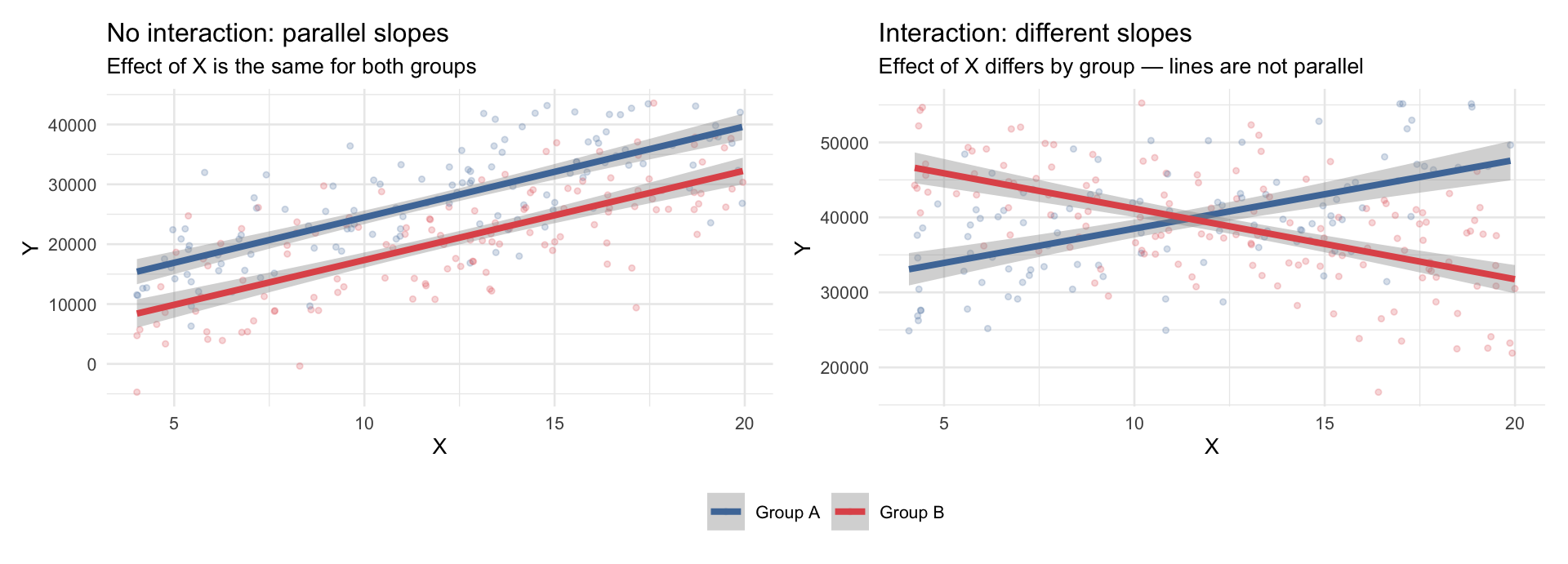
The key visual test for an interaction:

In the no-interaction model (Y ~ X + Z), the lines are parallel — the same slope for every group. In the interaction model (Y ~ X * Z), the slopes differ. The lines don’t need to cross — they just need to be non-parallel. Even a slight divergence (one slope steeper than the other) constitutes an interaction. The interaction term’s statistical significance tells us whether that difference in slopes is real or due to sampling noise.

The Interaction Model

To model an interaction, we add the product of the two predictors:

\[\hat{Y} = \alpha + \beta_1 X_1 + \beta_2 X_2 + \beta_3 (X_1 \times X_2)\]

What each coefficient means when $X_2$ is binary (0 = reference, 1 = other):

Coefficient	Meaning
$\beta_1$	Effect of $X_1$ on $Y$ for the reference group ($X_2 = 0$)
$\beta_2$	Difference in baseline $Y$ for $X_2 = 1$ vs. $X_2 = 0$ (when $X_1 = 0$)
$\beta_3$	The interaction: how much the effect of $X_1$ changes when $X_2 = 1$ instead of 0

Computing the effect for each group:

\[\text{Effect of } X_1 \text{ for reference group: } \hat\beta_1\] \[\text{Effect of } X_1 \text{ for key group: } \hat\beta_1 + \hat\beta_3\]

$\hat\beta_3$ is the difference in slopes between the two groups. If $\hat\beta_3 = 0$, the slopes are identical — no interaction.

In R: use * to include both main effects and the interaction term:

lm(Y ~ X1 * X2, data = my_data)    # = Y ~ X1 + X2 + X1:X2
lm(Y ~ X1 + X2 + X1:X2, data = my_data)  # same thing, written out

Always include lower-order (main effect) terms

A critical rule: whenever you include an interaction term $X_1 \times X_2$, you must also include the main effects $X_1$ and $X_2$ as separate terms in the same model. This is called the hierarchy principle.

Using Y ~ X1 * X2 in R enforces this automatically — it expands to Y ~ X1 + X2 + X1:X2. Never use Y ~ X1:X2 alone without the main effects — the model would be misspecified and the coefficients uninterpretable (the “effect of X₁ for the reference group” would lose its meaning without $\beta_1$ in the model).

Interpreting Interaction Terms

Continuous × Continuous
Continuous × Binary
Binary × Binary

Both X₁ and X₂ are continuous (e.g., occupational prestige × age → income).

\[\hat{Y} = \alpha + \beta_1 X_1 + \beta_2 X_2 + \beta_3 (X_1 \times X_2)\]

Effect of X₁ = $\beta_1 + \beta_3 X_2$ — the slope for X₁ depends on the value of X₂
Effect of X₂ = $\beta_2 + \beta_3 X_1$ — the slope for X₂ depends on the value of X₁

Interpreting direction

The sign of $\beta_3$ tells you how the relationship changes:

$\beta_3 > 0$: as $X_2$ increases, the effect of $X_1$ on $Y$ strengthens
$\beta_3 < 0$: as $X_2$ increases, the effect of $X_1$ on $Y$ weakens

Test of moderation: is $\beta_3$ statistically significantly different from zero?

Most common in sociology: continuous X₁, binary X₂ (e.g., sex, race indicator, treatment/control).

\[\hat{Y} = \alpha + \beta_1 X_1 + \beta_2 X_2 + \beta_3 (X_1 \times X_2)\]

Group	Full equation	Slope for X₁
$X_2 = 0$ (reference)	$\alpha + \beta_1 X_1$	$\beta_1$
$X_2 = 1$ (key group)	$(\alpha + \beta_2) + (\beta_1 + \beta_3) X_1$	$\beta_1 + \beta_3$
Difference in slopes		$\beta_3$

Our example: education × sex → income

$\beta_1$ = income return to education for men (reference)
$\beta_2$ = income difference between women and men when education = 0 — the intercept gap between the two regression lines. This is rarely a substantive quantity of interest; it just anchors where the women’s line starts. Use predicted values at realistic education levels to describe the actual income gap.
$\beta_3$ = how much women’s return differs from men’s — a positive $\beta_3$ means women benefit more per year; negative means women benefit less

Test of moderation: is $\beta_3$ statistically significantly different from zero?

Both X₁ and X₂ are binary (e.g., race × sex → income).

\[\hat{Y} = \alpha + \beta_1 X_1 + \beta_2 X_2 + \beta_3 (X_1 \times X_2)\]

X₁	X₂	Predicted Y
0	0	$\alpha$ (double reference)
1	0	$\alpha + \beta_1$
0	1	$\alpha + \beta_2$
1	1	$\alpha + \beta_1 + \beta_2 + \beta_3$

$\beta_3$ measures non-additivity: the effect of X₁ is different when X₂ = 1 vs. X₂ = 0
This is sometimes called a multiplicative interaction or a synergistic / suppressive effect

Worked Examples: Interaction Terms

Continuous × Continuous
Continuous × Binary
Binary × Binary

Model: lm(income91 ~ prestg80 * age) — does the income payoff of occupational prestige depend on career stage?

OLS: Income ~ Occupational Prestige × Age
	(1)
+ p < 0.1, * p < 0.05, p < 0.01, * p < 0.001
Intercept	32974.51***
	(6181.36)
Occupational Prestige	266.44+
	(139.53)
Age	-258.42*
	(130.31)
Prestige × Age	4.56
	(2.94)
Num.Obs.	2517
R2	0.041

Interpretation

Main effect of Occupational Prestige ($\beta_1$ = 266.44): this is the effect of prestige on income when age = 0 — a meaningless baseline. At the sample mean age (45.1 years), a one-unit increase in prestige is associated with $472.1 more income (266.44 + 4.56 × 45.1).

Main effect of Age ($\beta_2$ = -258.42): this is the effect of age on income when prestige = 0 — again, not meaningful on its own. At the sample mean prestige score (43.6), each additional year of age is associated with $-59.6 less income (-258.42 + 4.56 × 43.6).

Interaction ($\beta_3$ = 4.56): the prestige → income slope grows stronger as workers get older — prestige compounds over a career. In the margins plot on the next slide, this will appear as “steeper lines for older ages”.

High-level summary: Occupational prestige is positively associated with income, while age has a negative main effect on income at mean prestige levels. The positive interaction term suggests that the effect of prestige grows stronger with age — partially offsetting the negative age effect — but this interaction is not statistically significant, so the impact of prestige does not depend on age.

Model: lm(income91 ~ educ * sex_f) — does the income return to education differ by sex?

OLS: Income ~ Education × Sex
	(1)
+ p < 0.1, * p < 0.05, p < 0.01, * p < 0.001
Intercept	-6547
	(4848)
Years of Education	3836***
	(354)
Female	-6038
	(6928)
Education × Female	84
	(508)
Num.Obs.	2517
R2	0.089

Group	Slope for educ	Formula
Men (reference)	$\beta_1$	Baseline slope
Women	$\beta_1 + \beta_3$	Baseline + interaction
Difference	$\beta_3$	The interaction term itself

Interpretation

Main effect of Education ($\beta_1$ = $3,836): the income return to one additional year of education for men (the reference group). Because $X_2 = 0$ for men, this is a straightforward slope — men gain $3,836 per year of schooling.

Main effect of Female ($\beta_2$ = -$6,038): the income gap between women and men when education = 0 — the vertical distance between the two regression lines at their origin. This baseline intercept shift is not a substantively meaningful quantity on its own; use predicted values at realistic education levels to describe the actual income gap.

Interaction ($\beta_3$ = $84): women’s income return per additional year of education is $84 more than men’s. Men gain $3,836 per year; women gain $3,920 — a difference that is not statistically significant (p = 0.869).

High-level summary: Education is strongly positively associated with income for both men and women. The negative coefficient for women means they have lower predicted income at low levels of education. While women appear to have slightly higher returns to education than men (interaction term), this difference is not statistically significant.

Model: lm(income ~ Black * female) — does the racial income gap differ by sex?

OLS: Income ~ Race × Sex
	(1)
+ p < 0.1, * p < 0.05, p < 0.01, * p < 0.001
Intercept	64914***
	(663)
Black	-11319***
	(1127)
Women	-17639***
	(941)
Black × Women	2683
	(1657)
Num.Obs.	400
R2	0.601

Predicted incomes (2×2 table):

	White	Black
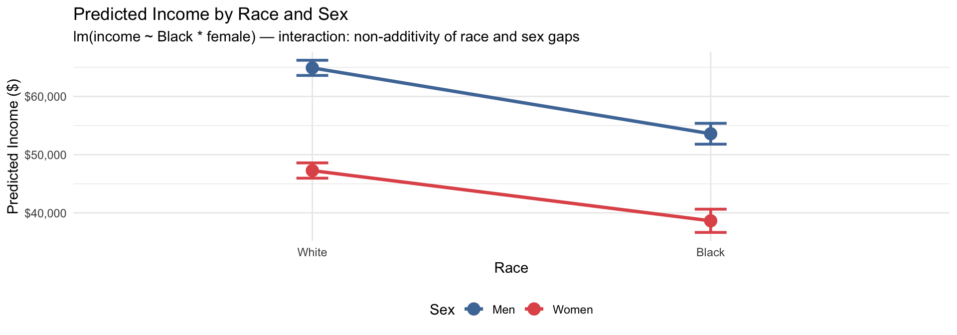
Men	$\alpha$ = $64,914	$\alpha + \beta_1$ = $53,595
Women	$\alpha + \beta_2$ = $47,275	$\alpha + \beta_1 + \beta_2 + \beta_3$ = $38,639

Where: $\alpha$ = $64,914, $\beta_1$ (Black) = −$11,319, $\beta_2$ (Women) = −$17,639, $\beta_3$ (interaction) = $2,683

Race gap within sex:

Among men: $64,914 − $53,595 = $11,319 ($\beta_1$)
Among women: $47,275 − $38,639 = $8,636 ($\beta_1 + \beta_3$)

Gender gap within race:

Among white workers: $64,914 − $47,275 = $17,639 ($\beta_2$)
Among Black workers: $53,595 − $38,639 = $14,956 ($\beta_2 + \beta_3$)

Race + gender gap (white men vs. Black women):

$64,914 − $38,639 = $26,275 ($\beta_1 + \beta_2 + \beta_3$)

Interpretation

Main effect of Race ($\beta_1$ = −$11,319): the income gap between white and Black men (the reference group for sex is men). Among men, Black workers earn $11,319 less than white workers.

Main effect of Sex ($\beta_2$ = −$17,639): the income gap between white men and white women (the reference group for race is white). Among white workers, women earn $17,639 less than men.

Interaction ($\beta_3$ = $2,683, p = 0.106): the additional income difference for Black women beyond what the two main effects predict additively. A positive $\beta_3$ means the combined penalty is smaller than the sum of the two gaps; negative means it is larger. This term is not statistically significant, so we cannot conclude that the racial income gap is meaningfully different for women versus men.

High-level summary: Both race and sex are independently associated with lower income. Black workers earn less than white workers, and women earn less than men. The interaction term–is not significant–but would suggest the two penalties do not simply add together for Black women.

Visualizing Interaction Terms

Continuous × Continuous
Continuous × Binary
Binary × Binary

Model: lm(income91 ~ prestg80 * age) — does the income payoff of occupational prestige depend on career stage?

People often visualize the dependency of one variable on the other by breaking the variable of interest into different groups. Here, age is broken into three relevant analytical groups; if there are no clear breaks, use standard deviations.

Code

p_int <- ggpredict(model_prestige, terms = c("prestg80", "age [30, 45, 60]")) |>
  ggplot(aes(x = x, y = predicted, color = group, fill = group)) +
  geom_ribbon(aes(ymin = conf.low, ymax = conf.high), alpha = 0.15, color = NA) +
  geom_line(linewidth = 1.4) +
  scale_color_manual(
    values = c("#E15759", "#4E79A7", "#59A14F"),
    labels = c("Age 30", "Age 45", "Age 60"),
    name   = "Age"
  ) +
  scale_fill_manual(
    values = c("#E15759", "#4E79A7", "#59A14F"),
    labels = c("Age 30", "Age 45", "Age 60"),
    name   = "Age"
  ) +
  scale_y_continuous(labels = scales::dollar_format(big.mark = ",")) +
  labs(
    title    = "With interaction",
    subtitle = "Slope varies by age — does prestige compound over a career?",
    x = "Occupational Prestige Score",
    y = "Predicted Income ($)"
  ) +
  theme_minimal(base_size = 10) +
  theme(legend.position = "bottom")

p_int

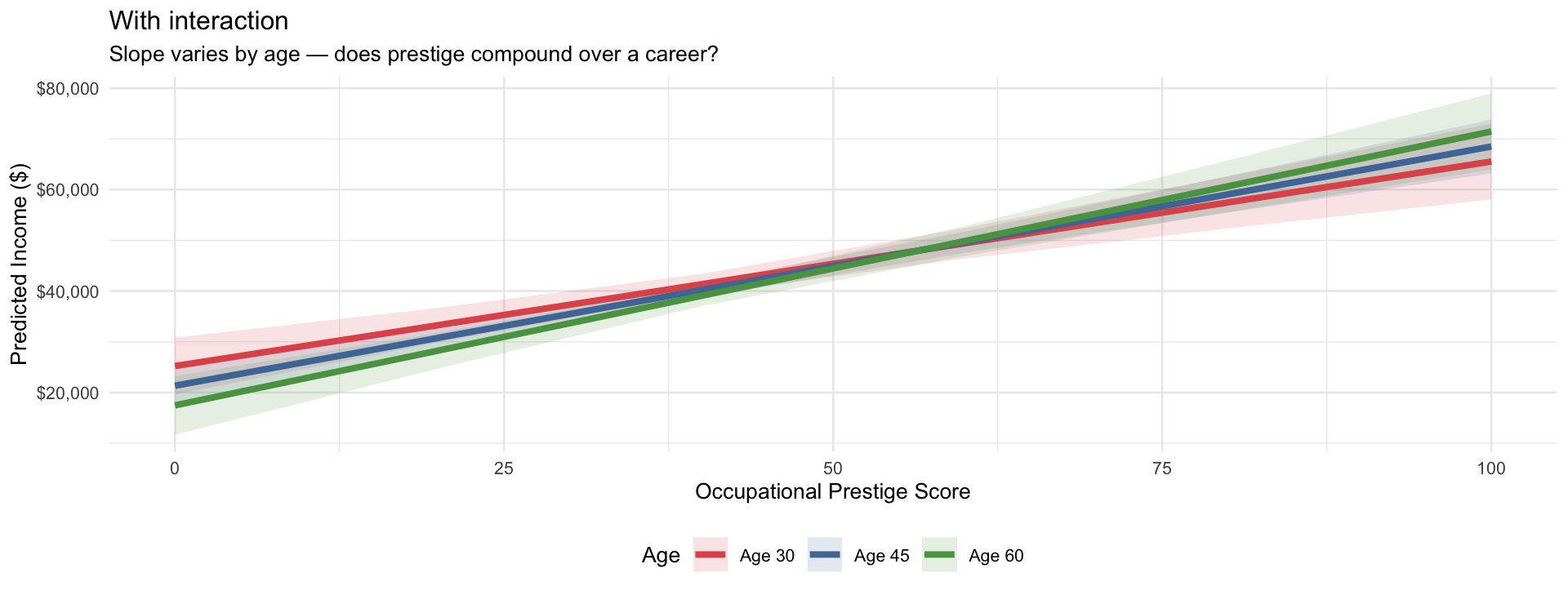
Reading the plot

Each line shows the prestige → income slope at a different career stage (30, 45, 60).

Parallel lines = no interaction, prestige pays off the same regardless of age.
Diverging lines = interaction, the prestige premium grows (or shrinks) with age.

Here we see steeper lines for older ages as the coefficent for the interaction suggests, but the coefficient is not significant. Always check the confidence intervals: the interaction is significant wherever there is no overlap – no real difference in this figure.

Model: lm(income91 ~ educ * sex_f) — does the income return to education differ by sex?

This is simpler to visualize since the categories are already decided for you, unlike with a continuous by continuous interaction.

Code

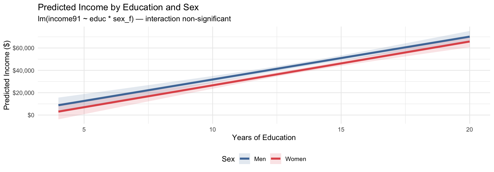
ggpredict(model_interact, terms = c("educ [4:20 by=0.5]", "sex_f")) |>
  ggplot(aes(x = x, y = predicted, color = group, fill = group)) +
  geom_ribbon(aes(ymin = conf.low, ymax = conf.high), alpha = 0.15, color = NA) +
  geom_line(linewidth = 1.4) +
  scale_color_manual(
    values = c("male" = "#4E79A7", "female" = "#E15759"),
    labels = c("Men", "Women"), name = "Sex"
  ) +
  scale_fill_manual(
    values = c("male" = "#4E79A7", "female" = "#E15759"),
    labels = c("Men", "Women"), name = "Sex"
  ) +
  scale_y_continuous(labels = scales::dollar_format(big.mark = ",")) +
  labs(
    title    = "Predicted Income by Education and Sex",
    subtitle = "lm(income91 ~ educ * sex_f) — interaction non-significant",
    x = "Years of Education",
    y = "Predicted Income ($)"
  ) +
  theme_minimal(base_size = 11) +
  theme(legend.position = "bottom")

Reading the plot

The two lines show the income slope for men (blue) and women (red) across years of education. We know from the model output that the interaction is not significant and the lines are basically parallel. Additionally, the CIs overlap at nearly all points.

Model: lm(income ~ Black * female) — does the racial income gap differ by sex?

Code

ggpredict(model_bb, terms = c("Black", "female")) |>
  ggplot(aes(x = x, y = predicted, color = group, group = group)) +
  geom_point(size = 4) +
  geom_line(linewidth = 1.2) +
  geom_errorbar(aes(ymin = conf.low, ymax = conf.high), width = 0.08, linewidth = 1.0) +
  scale_color_manual(
    values = c("Men" = "#4E79A7", "Women" = "#E15759"), name = "Sex"
  ) +
  scale_y_continuous(labels = scales::dollar_format(big.mark = ",")) +
  labs(
    title    = "Predicted Income by Race and Sex",
    subtitle = "lm(income ~ Black * female) — interaction: non-additivity of race and sex gaps",
    x = "Race",
    y = "Predicted Income ($)"
  ) +
  theme_minimal(base_size = 11) +
  theme(legend.position = "bottom")

Reading the plot

The drop from White to Black on each line represents the racial income gap. Parallel lines mean the gap is identical for men and women — no interaction. Non-parallel lines suggest the gap differs by sex.

Black × Women ($\beta_3$ = $2,683, p = 0.106) is not statistically significant — we cannot conclude that the racial income gap actually differs by sex. Any non-parallelism visible in the plot is consistent with sampling noise.

Running Example: Does Education Pay Off Equally?

Research question: Does each additional year of education translate into the same income gain for men and women?

Why this matters sociologically:

A central debate in stratification research: Do women earn less simply because they have less education? Or does the return to education itself differ by gender — meaning each year of education is worth more in the labor market for men than for women?

If $\beta_3 < 0$ (education × female), this is evidence of structural inequality: even with identical credentials, women receive a lower wage premium per year of schooling.

# Without interaction: assumes same education slope for men and women
model_main <- lm(income91 ~ educ + sex_f, data = attain_sub)

# With interaction: allows slopes to differ by sex
model_interact <- lm(income91 ~ educ * sex_f, data = attain_sub)

# Extract key coefficients
coef(model_interact)

     (Intercept)             educ      sex_ffemale educ:sex_ffemale 
     -6547.43864       3836.33531      -6037.51913         83.89174

Interaction Model Results

Model Table
Reading the Coefficients
Predicted Incomes
Slopes Plot

Code

modelsummary(
  list("No Interaction"   = model_main,
       "With Interaction" = model_interact),
  coef_rename = c("(Intercept)"      = "Intercept",
                  "educ"             = "Years of Education",
                  "sex_ffemale"      = "Female",
                  "educ:sex_ffemale" = "Education × Female"),
  stars   = TRUE,
  fmt     = 0,
  title   = "OLS: Income ~ Education × Sex",
  gof_map = c("nobs", "r.squared", "adj.r.squared")
)

OLS: Income ~ Education × Sex
	No Interaction	With Interaction
+ p < 0.1, * p < 0.05, p < 0.01, * p < 0.001
Intercept	-7092*	-6547
	(3557)	(4848)
Years of Education	3877***	3836***
	(254)	(354)
Female	-4919***	-6038
	(1472)	(6928)
Education × Female		84
		(508)
Num.Obs.	2517	2517
R2	0.089	0.089
R2 Adj.	0.088	0.088

Interpreting the interaction model:

From the regression output:

Education (3836): Effect of each year of education for men (the reference group)
Female (-$6,038): Difference in baseline income for women vs. men at education = 0 — not substantively meaningful on its own
Education × Female (84): Women receive $84 more per additional year of education compared to men — this is the interaction

Slopes by group:

Group	Income return per year of education
Men	$3,836
Women	$3,836 + (84) = $3,920
Difference	84 (p = 0.869)

High-level summary: Education is strongly positively associated with income for both men and women. The negative coefficient for women means they have lower predicted income at low levels of education. While women appear to have slightly higher returns to education than men (interaction term), this difference is not statistically significant.

We can also calculate predicted incomes for specific profiles:

profiles <- tibble(
  educ  = c(12, 12, 16, 16),
  sex_f = c("male", "female", "male", "female")
)

profiles |>
  mutate(predicted_income = predict(model_interact, newdata = profiles)) |>
  mutate(predicted_income = scales::dollar(round(predicted_income)))

# A tibble: 4 × 3
   educ sex_f  predicted_income
  <dbl> <chr>  <chr>           
1    12 male   $39,489         
2    12 female $34,458         
3    16 male   $54,834         
4    16 female $50,139

The income gap by education level:

At high school education (12 years): men earn $39,489 vs. women $34,458 — a gap of $5,031
At college education (16 years): men earn $54,834 vs. women $50,139 — a gap of $4,695

If the interaction term is negative, the gender wage gap widens with education — more education amplifies inequality, not diminishes it.

Code

ggpredict(model_interact, terms = c("educ [4:20 by=0.5]", "sex_f")) |>
  ggplot(aes(x = x, y = predicted, color = group, fill = group)) +
  geom_ribbon(aes(ymin = conf.low, ymax = conf.high), alpha = 0.15, color = NA) +
  geom_line(linewidth = 1.4) +
  scale_color_manual(values = c("male" = "#4E79A7", "female" = "#E15759"),
                     labels = c("Men", "Women"), name = "Sex") +
  scale_fill_manual(values  = c("male" = "#4E79A7", "female" = "#E15759"),
                    labels  = c("Men", "Women"), name = "Sex") +
  scale_y_continuous(labels = scales::dollar_format(big.mark = ",")) +
  labs(
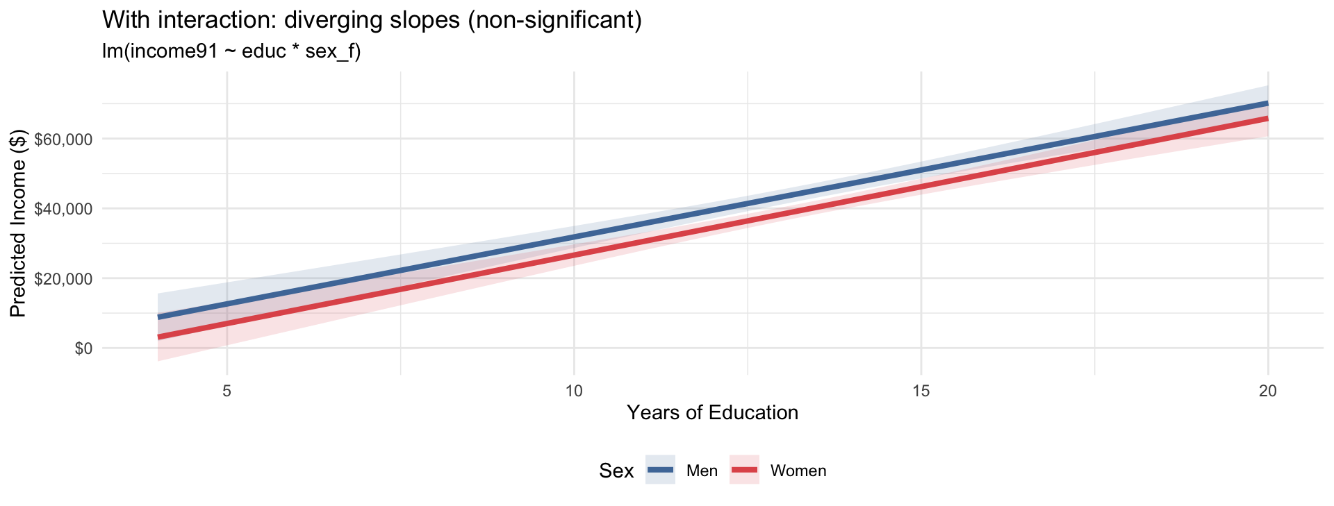
    title    = "With interaction: diverging slopes (non-significant)",
    subtitle = "lm(income91 ~ educ * sex_f)",
    x = "Years of Education", y = "Predicted Income ($)"
  ) +
  theme_minimal(base_size = 11) +
  theme(legend.position = "bottom")

What to look for in an interaction plot:

Line slope: A steeper line = higher income return per year of education for that group.

Line gap at each X value: The vertical distance between men’s and women’s predicted incomes. If the lines are parallel (same slope), the gap is constant; if one line’s slope is steeper, the gap widens or decreases with education. Hard to tell in this case.

Confidence ribbons: Overlapping ribbons signal uncertainty about whether the two slopes are truly different. The formal test is the p-value on the interaction term. In this case, they mostly overlap.

Testing and Reporting the Interaction

Is the interaction statistically significant?

The interaction term $\hat\beta_3$ has its own standard error, t-statistic, and p-value in the regression output. This tests:

\[H_0: \beta_3 = 0 \quad \text{(no interaction — slopes are the same for both groups)}\] \[H_A: \beta_3 \neq 0 \quad \text{(slopes differ between groups)}\]

In our example: p = 0.869 for the education × female interaction term.

Reporting checklist for an interaction result:

State the substantive question: Does the effect of X on Y vary by Z?
Report the interaction coefficient: $\hat\beta_3$ = 84 ($p = 0.869$)
State the group-specific slopes: men = $3,836/year; women = $3,920/year
Show the visualization: margins plot with two lines, CIs
Interpret substantively: what does it mean that the slopes differ? Connect to theory.

A note on statistical power

Interaction terms are often hard to detect — you need a large sample and a reasonably strong moderating effect. A non-significant interaction term does not necessarily mean “no interaction exists in the population.” It may mean the study is underpowered. Be cautious about drawing strong null conclusions from a single insignificant $\hat\beta_3$.

Interactions in Logistic Regression

Interaction terms work the same way in logistic regression — same syntax, same logic. Let’s look at the interaction of education and sex on likely union membership.

Model Table
Visualization

Code

attain_logit <- attain |>
  filter(!is.na(union_member), !is.na(educ), !is.na(sex_f))

# Logistic regression with interaction
model_logit_int <- glm(union_member ~ educ * sex_f,
                       family = binomial,
                       data   = attain_logit)

modelsummary(model_logit_int,
             exponentiate = TRUE,
             coef_rename  = c("(Intercept)"      = "Intercept",
                              "educ"             = "Years of Education",
                              "sex_ffemale"      = "Female",
                              "educ:sex_ffemale" = "Education × Female"),
             stars   = TRUE,
             title   = "Logistic Regression with Interaction (Odds Ratios)",
             gof_map = c("nobs", "AIC"))

Logistic Regression with Interaction (Odds Ratios)
	(1)
+ p < 0.1, * p < 0.05, p < 0.01, * p < 0.001
Intercept	0.337**
	(0.120)
Years of Education	0.931**
	(0.025)
Female	0.018***
	(0.012)
Education × Female	1.278***
	(0.058)
Num.Obs.	2985

Interpretation

Main effect of Education (OR = 0.931, p < 0.01): for men (the reference group), each additional year of education multiplies the odds of union membership by 0.931. An OR < 1 means education is negatively associated with union membership among men. This effect is statistically significant.

Main effect of Female (OR = 0.018, p < 0.001): the odds ratio comparing women to men when education = 0 — a baseline intercept shift with no direct substantive meaning. Interpret the sex difference through predicted probabilities at realistic education values instead. This effect is statistically significant.

Interaction: Education × Female (OR = 1.278, p < 0.001): the ratio of education’s OR for women to men. An OR > 1 means each year of education multiplies women’s odds by more than men’s — the education effect is stronger for women. This interaction is statistically significant.

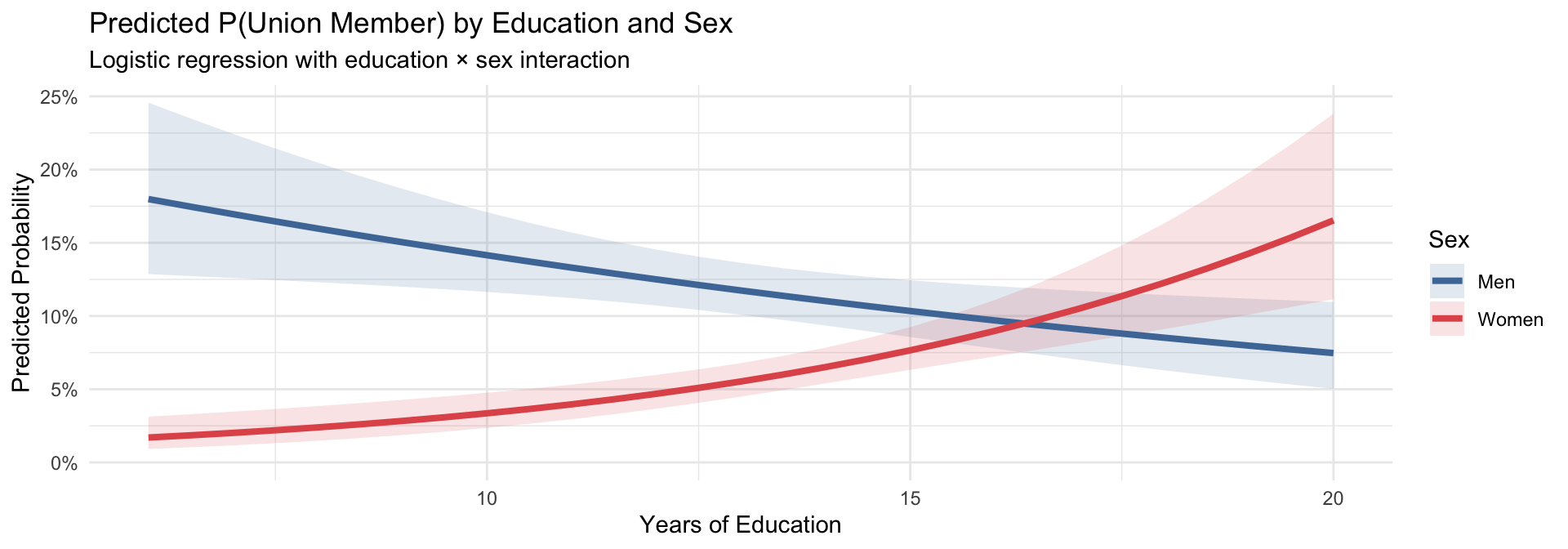
High-level summary: Education decreases the odds of union membership for men. The interaction term tells us whether that effect differs for women — since it’s positive, the effect of education is positive for women, which we’ll see clearly in the margins plot.

Code

ggpredict(model_logit_int, terms = c("educ [6:20 by=0.5]", "sex_f")) |>
  (\(pred) {
    ggplot(pred, aes(x = x, y = predicted, color = group, fill = group)) +
      geom_ribbon(aes(ymin = conf.low, ymax = conf.high), alpha = 0.15, color = NA) +
      geom_line(linewidth = 1.4) +
      scale_color_manual(values = c("male" = "#4E79A7", "female" = "#E15759"),
                         labels = c("Men", "Women"), name = "Sex") +
      scale_fill_manual(values  = c("male" = "#4E79A7", "female" = "#E15759"),
                        labels  = c("Men", "Women"), name = "Sex") +
      scale_y_continuous(labels = scales::percent_format(accuracy = 1),
                         limits = c(0, NA)) +
      labs(
        title    = "Predicted P(Union Member) by Education and Sex",
        subtitle = "Logistic regression with education × sex interaction",
        x = "Years of Education",
        y = "Predicted Probability"
      ) +
      theme_minimal(base_size = 11)
  })()

Why are the curves S-shaped — and what does the interaction mean?

The S-curve is not from a quadratic term. It comes from logistic regression itself: the model estimates odds ratios on a multiplicative scale, but ggpredict() converts those to probabilities (which must stay between 0 and 1). That conversion always produces an S-shaped (sigmoid) curve.

Reading the interaction:

The interaction OR (Education × Female = 1.278, p < 0.001) is statistically significant. An OR > 1 means each year of education multiplies women’s odds by more than men’s (specifically, by a factor of 1.278 relative to men’s OR of 0.931) — so the lines diverge as education rises. This is why the probability curves diverge at higher education levels in the plot.

Questions?

Reading: Thompson & Keith (2001)

Interactions in a classic race & gender study

“The Blacker the Berry” — Overview

Thompson, M.S. & Keith, V.M. (2001). The Blacker the Berry: Gender, Skin Tone, Self-Esteem, and Self-Efficacy. Gender & Society, 15(3), 336–357.

Research question: How does skin tone affect self-esteem and self-efficacy among Black Americans — and does this effect depend on gender?

Studies colorism: the privileging of lighter skin tones within racial groups — a legacy of slavery, segregation, and Eurocentric beauty standards
Uses OLS regression with continuous × continuous interaction terms — skin tone × income, attractiveness, and weight
Key finding: the effect of skin tone on well-being is conditional on social resources — and the relevant resources differ for Black women vs. Black men

Why this paper for interactions week?

Thompson & Keith use continuous × continuous interactions to show that skin tone’s effect on self-esteem is not fixed — it depends on what social resources you have (income, attractiveness for women; weight for men). This is exactly the moderation logic we covered in Part 2: the X → Y relationship changes depending on Z. The paper also models how to justify an interaction theoretically before testing it empirically.

Research Design

Data & Sample
Variables

Data: National Survey of Black Americans (NSBA), a nationally representative survey of Black adults
Sample: Black Americans aged 18+ — Wave I (1979–80) and Wave IV (1992)
Context: 1970s–80s US — ongoing de facto racial stratification and deeply gendered standards of beauty

Role	Variable	Measurement
Outcome 1	Self-esteem	Multi-item scale (Rosenberg items)
Outcome 2	Self-efficacy	Multi-item scale (locus of control items)
Key predictor (X₁)	Skin tone	Interviewer-rated, 5-point scale (1 = very light, 5 = very dark)
Main Moderator (Sample)	Gender	Binary: female / male
Secondary Moderators (X₂)	Income, Attractiveness, Weight	Continuous measures
Interaction	Skin tone × Income, × Attractiveness, × Weight,	Tests whether the skin tone effect differs by Income, Attractiveness, and weight by gender
Controls	Education, age, marital status, region	Individual characteristics

Connecting to today’s framework:

Their regression is equivalent to a three way interaction, for example:

lm(self_esteem ~ skin_tone * gender * income + age + ...,
   data = nsba)

Key Results: The Skin Tone × Gender Interaction

What They Found
Simplified Results Table
Discussion & Interpretation (pp. 351–354)
Lessons for Your Research

The core finding (Results pp. 349–351):

Thompson & Keith run separate OLS models for women and men. Rather than one skin-tone × gender * third moderateor term, they find continuous × continuous interactions within each gender’s model — the effect of skin tone depends on other social resources. To bear there out, they break make cut points by one of the continuous variables for comparison.

Women’s self-esteem (Table 4):

Skin tone × Income: b¹ = −.035* — darker skin lowers self-esteem most for low-income women; the effect disappears at high income
Skin tone × Attractiveness: b¹ = −.113* — darker skin lowers self-esteem most for women rated low in attractiveness

Men’s self-esteem and self-efficacy (Table 4):

Skin tone × Weight → self-esteem: b¹ = +.274* — darker skin hurts self-esteem for low-weight men but helps for high-weight men
Skin tone × Weight → self-efficacy: b¹ = +.188† — same moderator, same direction: weight conditions how skin tone relates to self-efficacy

The bigger picture: skin tone’s relationship with well-being is highly conditional — it depends on what social resources you have. And those resources differ by gender, which is why the pattern looks so different for women vs. men.

Thompson & Keith (2001), Table 4 — significant interaction effects with simple slopes at low, average, and high values of the moderator. Models run separately by gender.

Model	Interaction	b¹ (int.)	Moderator level	b² (skin tone slope)
Women Self-Esteem	Skin Tone × Income	−.035*	Low income	+.376*
			Average income	+.185*
			High income	−.005
	Skin Tone × Attractiveness	−.113*	Low attractiveness	+.350**
			Average attractiveness	+.184*
			High attractiveness	+.018
Men Self-Esteem	Skin Tone × Weight	+.274*	Low weight	−1.009*
			Average weight	+.092
			High weight	+1.192**
Men Self-Efficacy	Skin Tone × Weight	+.188†	Low weight	−.545
			Average weight	+.210†
			High weight	+.965*

*p ≤ .05; **p ≤ .01; †p ≤ .10. b¹ = interaction term coefficient. b² = simple slope of skin tone at each moderator level. From Thompson & Keith (2001), Table 4.

How to read this table:

b¹ is the interaction coefficient — it tests whether the skin tone slope changes as the moderator increases (negative b¹ = the effect weakens as the moderator rises). b² gives the simple slope at specific moderator values: the effect of skin tone on self-esteem for women at low income, etc. The skin tone slope is significant at low and average income/attractiveness, but vanishes at high levels — darker skin penalizes women’s self-esteem only when they lack other social resources.

Why does gender moderate the skin tone effect?

Thompson & Keith argue that American society applies gendered standards of beauty that tie women’s (but not men’s) social worth to physical appearance. Darker-skinned Black women are evaluated against a Eurocentric beauty ideal they are structurally excluded from. For Black men, self-concept is more tied to occupational achievement and social status — which are less directly linked to skin tone.

This is a structural interpretation of a statistical interaction. The interaction term is not just a number; it reflects deep patterns of racial and gender inequality in how society evaluates worth and confers status.

What Thompson & Keith model for writing up interactions:

Justify the interaction theoretically first — they explain why they expect gender to moderate the skin tone effect before showing the numbers
Report group-specific slopes — not just “the interaction is significant” but “for women, the slope is X; for men, it is Y”
Interpret substantively in the Discussion — what does the interaction mean about social structure?
Use the interaction to test structural arguments — the point is not just statistics, it’s theory

Connecting the Reading to Today

Thompson & Keith concept	Our framework
Run separate models for women and men	Stratified analysis — or a single model with gender interactions
Different moderators for women vs. men	Theory first: income/attractiveness matter for women’s status; weight for men’s
Connects to colorism + gender theory	Substantive interpretation of $\beta_3$ — not just a number

For your research paper:

T&K’s approach models what good interaction research looks like: they specify a theoretically justified moderator (not just “does sex moderate everything?”), run the interaction, report simple slopes at meaningful moderator values, and interpret the result in terms of social structure. The same logic applies to your interaction hypothesis.

Questions?

Key Takeaways

Part 1 — Controls
Part 2 — Interactions

Confounders are variables that affect both X and Y, creating a spurious association between them
Controlling for Z (Y ~ X + Z) asks: “Among people with the same Z, what is the relationship between X and Y?”
The education coefficient can change when we add controls — that change tells us how much the confounder was biasing the original estimate
Only control for true confounders: variables prior to X and Y that have causal paths to both
Do NOT control for mediators (variables caused by X that cause Y) — we’ll cover mediation next week

An interaction occurs when Z moderates the effect of X on Y: the X → Y relationship differs across levels of Z
Add an interaction with lm(Y ~ X * Z) — R automatically includes X, Z, and X:Z
Always interpret main and interaction effect together, how you do this varies slighly by measurement of interacting variables (binary vs continuous)
Always visualize with ggpredict(model, terms = c("X", "Z")) — parallel vs. crossing slope, check the CIs
Same logic applies to logistic regression with glm(..., family = binomial)
Interpret interactions substantively — connect to theory, not just p-values

Without interaction	With interaction
`Y ~ X + Z` → parallel slopes	`Y ~ X * Z` → different slopes
Effect of X same for all Z	Effect of X varies by Z
Use when no moderation expected	Use when theory predicts heterogeneity

Why This Matters for Your Research Paper

Should you include an interaction in your final paper?

Add a control variable if: There is a theoretically justified confounding variable you want to rule out as an alternative explanation for your X → Y relationship.

Add an interaction if: You have a specific theoretical argument that the X → Y relationship varies across groups or contexts. The interaction is the test of that argument.

Don’t add either just because you can. Every model extension should be motivated by theory and research question, not by fishing for significant coefficients.

Thompson & Keith as a model:

Their paper shows how to: (1) justify the interaction based on theory, (2) run the regression with the interaction term, (3) report and interpret group-specific slopes, and (4) connect the result back to the theoretical argument. The same four steps apply to your paper.

Questions?

Assignments

Weekly Assignment #11

Canceled to focus on final paper and final exam

Also upcoming:

Revised Proposal with Outline — Due Thursday, April 16
- Describe whether your final analysis includes any control variables or interaction hypotheses
In-class presentations — April 28/May 5
Final paper — Due Thursday, May 7

Coefficient	Meaning
\(\beta_1\)	Effect of \(X_1\) on \(Y\) for the reference group (\(X_2 = 0\))
\(\beta_2\)	Difference in baseline \(Y\) for \(X_2 = 1\) vs. \(X_2 = 0\) (when \(X_1 = 0\))
\(\beta_3\)	The interaction: how much the effect of \(X_1\) changes when \(X_2 = 1\) instead of 0

Group	Full equation	Slope for X₁
\(X_2 = 0\) (reference)	\(\alpha + \beta_1 X_1\)	\(\beta_1\)
\(X_2 = 1\) (key group)	\((\alpha + \beta_2) + (\beta_1 + \beta_3) X_1\)	\(\beta_1 + \beta_3\)
Difference in slopes		\(\beta_3\)

X₁	X₂	Predicted Y
0	0	\(\alpha\) (double reference)
1	0	\(\alpha + \beta_1\)
0	1	\(\alpha + \beta_2\)
1	1	\(\alpha + \beta_1 + \beta_2 + \beta_3\)

	White	Black
Men	\(\alpha\) = $64,914	\(\alpha + \beta_1\) = $53,595
Women	\(\alpha + \beta_2\) = $47,275	\(\alpha + \beta_1 + \beta_2 + \beta_3\) = $38,639