Week 11

Sociology 106: Quantitative Sociological Methods

March 31, 2026

Agenda

Housekeeping:

  • HW #8, HW #9, Revised Proposal with Outline

Statistical content — four parts:

  • Part 1: Outcome variables and key predictors — what are we trying to explain?
  • Part 2: From correlation to regression — estimating the magnitude of a linear relationship
  • Part 3: Regression with categorical predictors — dummy variables and baseline categories
  • Part 4: OLS assumptions and multiple regression

In-class lab:

  • Applying OLS regression to GSS data

Housekeeping

Weekly Assignment #8

  • Due Thursday, April 2 — hypothesis testing from Week 9

Weekly Assignment #9

  • Due Thursday, April 9
  • Run an OLS regression on your research dataset — today’s lecture covers everything you need
  • Uses modelsummary() for a clean regression table (covered today)
  • If using a categorical predictor, use fct_relevel() to set a baseline category (covered today)

Revised Proposal with Outline

  • Due Thursday, April 16
  • Should now describe the statistical techniques you plan to use — including regression!
  • Come to office hours if you need help connecting your research question to a regression model

Where We Are in the Course

  • Week 9: Hypothesis testing — is there a relationship, or is it just chance?
  • This week (Week 11): Linear regression — how strong is the relationship, and in what direction?
  • Week 12: Logistic regression — predicting binary outcomes
  • Week 13: Extensions — multiple controls, more complex models

The big picture: from “yes or no” to “how much?”

Last week we answered: “Is there a statistically significant relationship?” Today’s tool — regression — gives a quantitative answer: “For every one-unit increase in X, how much does Y change on average?”

Part 1: Outcome Variables and Key Predictors

What are we trying to explain, and with what?

Two Variables, Two Roles

Every regression analysis has variables playing two distinct roles:

The outcome variable — what you are trying to explain or predict

  • Also called: dependent variable (DV), response variable, Y
  • This is the phenomenon your research question is about – the thing that is effected

The predictor — what you are using to explain the outcome

  • Also called: key independent variable (key IV), explanatory variable, X
  • This is the main theoretical variable your hypothesis is about – the thing that does the affecting

These labels reflect your theory, not your data:

Calling one variable the “outcome” and another the “predictor” encodes your theoretical argument about which variable explains which. Regression is a tool for formalizing that argument quantitatively.

Language Matters

You’ll encounter many terms for the same concept — here’s a cheat sheet:

Term What it means Also called
Outcome variable What you are trying to explain Dependent variable (DV), Y, response variable
Key predictor Your main explanatory variable Key IV, key independent variable, X
Control variable Additional IV included to rule out alternatives Covariate


In your research paper:

Your paper proposal asked you to identify your key independent and dependent variables. These map directly onto key predictor and outcome variable in regression. Today you learn to formally estimate the relationship between them.

Setting Up Your Research Question

Before running any regression, be explicit about your variables and expectations:

Your research question should name both roles:

“How does occupational prestige impact household income?”

  • Outcome variable (Y): income91 — household income, in dollars — what we’re explaining
  • Key predictor (X): prestg80 — occupational prestige score — our main theoretical variable

Why income as the outcome?

We have theoretical reasons to believe occupational status drives income (not the reverse). The direction of influence determines which variable goes on which side of the regression equation.

Write out your hypothesis before looking at the data:

\[H_0: \beta_{\text{prestige}} = 0 \quad \text{(prestige has no effect on income)}\]

\[H_1: \beta_{\text{prestige}} > 0 \quad \text{(higher prestige → higher income)}\]

This is a one-tailed test — theory strongly predicts the direction (positive).

In most cases, we’ll default to two-tailed unless we have strong prior theoretical reason for directionality.

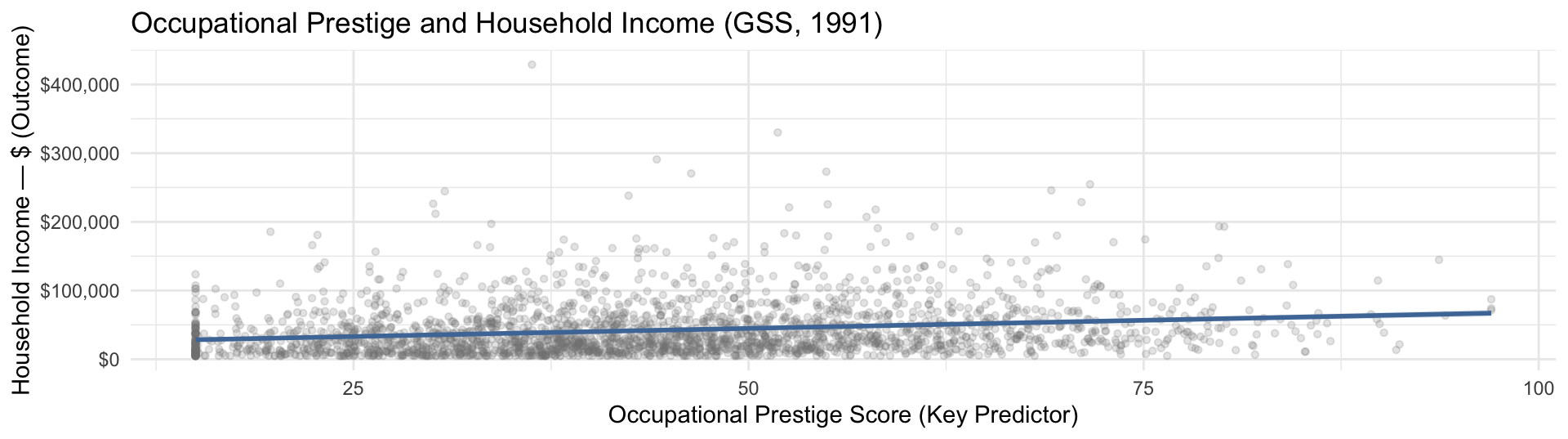
Always plot your variables before running a regression:

ggplot(attain_reg, aes(x = prestg80, y = income91)) +
  geom_point(alpha = 0.2, color = "gray50", size = 1.2) +
  geom_smooth(method = "lm", se = TRUE, color = "#4E79A7",
              fill = "#4E79A7", alpha = 0.15) +
  scale_y_continuous(labels = scales::dollar_format()) +
  labs(title = "Occupational Prestige and Household Income (GSS, 1991)",
       x = "Occupational Prestige Score (Key Predictor)",
       y = "Household Income — $ (Outcome)") +
  theme_minimal(base_size = 11)

Questions?

Part 2: From Correlation to Regression

From “is there a relationship?” to “how strong is it?”

What Correlation Tells Us — and What It Doesn’t

A correlation coefficient (r) describes direction and strength:

r Strength
r ≈ 0.3 Weak
r ≈ 0.5 Moderate
r ≈ 0.8 Strong

But correlation cannot answer:

  • How many dollars does income increase per one-point gain in occupational prestige?
  • What is the predicted income for someone with a prestige score of 50?
  • Is this relationship significant after controlling for sex?

The key limitation:

Two datasets can have the same correlation (r = 0.82) but completely different slopes — different magnitudes, different units, different practical meanings.

Regression gives us the slope — the actual quantitative size of the relationship in the units of Y per unit of X.

The Linear Regression Model

For any value \(x\) of the key predictor, the expected value of the outcome is:

\[E[Y \mid x] = \alpha + \beta x\]

Symbol Name Meaning
\(E[Y \mid x]\) Conditional mean Expected (average) value of outcome \(Y\) when \(X = x\)
\(\alpha\) Intercept Predicted value of \(Y\) when \(X = 0\) — the baseline anchor
\(\beta\) Slope Average change in \(Y\) for a one-unit increase in \(X\)

In practice, we estimate from sample data:

\[y_i = a + bx_i + e_i\]

  • \(a\) = estimated intercept (sample estimate of \(\alpha\))
  • \(b\) = estimated slope (sample estimate of \(\beta\)) — this is the key number
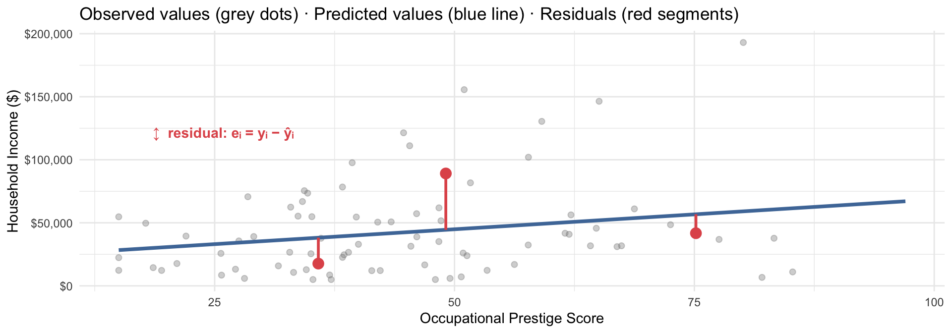
  • \(e_i\) = residual for observation \(i\) — the gap between observed \(y_i\) and predicted \(\hat{y}_i\)

OLS (ordinary least squares) chooses \(a\) and \(b\) to minimize:

\[\text{RSS} = \sum_{i=1}^{n} e_i^2 = \sum_{i=1}^{n} (y_i - a - bx_i)^2\]

Why square? Prevents cancellation, penalizes large misses, and produces a unique closed-form solution.

Observed vs. Predicted Values

Note

Residual \(e_i = y_i - \hat{y}_i\): how far each observation is from the line. OLS minimizes the sum of squared residuals — hence “ordinary least squares.”

Running OLS in R

The lm() function runs OLS regression:

lm(outcome ~ key_predictor, data = your_data)
  • The variable on the left of ~ is always the outcome (Y)
  • The variable on the right is the key predictor (X)

Our example:

# Filter to complete cases
attain_reg <- attain |> filter(!is.na(prestg80), !is.na(income91))

# Fit the OLS model — outcome ~ key_predictor
model_biv <- lm(income91 ~ prestg80, data = attain_reg)
summary(model_biv)

Call:
lm(formula = income91 ~ prestg80, data = attain_reg)

Residuals:
   Min     1Q Median     3Q    Max 
-53305 -24664 -10902  12726 390467 

Coefficients:
            Estimate Std. Error t value            Pr(>|t|)    
(Intercept) 21273.31    2134.09   9.968 <0.0000000000000002 ***
prestg80      472.13      45.94  10.277 <0.0000000000000002 ***
---
Signif. codes:  0 '***' 0.001 '**' 0.01 '*' 0.05 '.' 0.1 ' ' 1

Residual standard error: 37680 on 2525 degrees of freedom
Multiple R-squared:  0.04015,   Adjusted R-squared:  0.03977 
F-statistic: 105.6 on 1 and 2525 DF,  p-value: < 0.00000000000000022

modelsummary() from the modelsummary package produces a cleaner, publication-ready table — use this in hw9:

modelsummary(model_biv,
             coef_rename = c("(Intercept)" = "Intercept",
                             "prestg80"    = "Prestige Score"),
             stars   = TRUE,
             title   = "OLS: Household Income ~ Occupational Prestige",
             gof_map = c("nobs", "r.squared", "adj.r.squared"))
OLS: Household Income ~ Occupational Prestige
 (1)
Intercept 21273.309***
(2134.090)
Prestige Score 472.133***
(45.943)
Num.Obs. 2527
R2 0.040
R2 Adj. 0.040
+ p < 0.1, * p < 0.05, ** p < 0.01, *** p < 0.001

What each row means:

Intercept: Predicted income when prestige = 0. Not substantively meaningful for prestige (no one has a prestige score of 0) — just the mathematical anchor for the line.

Prestige Score (slope): For each additional point in occupational prestige, household income is predicted to be about $472 higher, on average. This is your key result.

Standard error: How precisely we’ve estimated the slope. Smaller SE → more confidence.

Stars / p-value: Is the slope significantly different from zero? Here, \(p < 0.001\) — we strongly reject \(H_0: \beta = 0\).

R²: Occupational prestige explains about 4% of the variation in household income. Report and interpret this in hw9.
Coefficients and Hypothesis Tests

Every OLS coefficient has its own built-in hypothesis test:

\[t = \frac{b}{SE(b)}, \quad \text{compared to } t\text{-distribution with } df = n - k - 1\]

This is identical to Week 9’s t-test logic — the only thing new is what we’re testing

# Each column has a precise meaning:
#   Estimate    = the coefficient (b)
#   Std. Error  = SE(b) — precision of the estimate
#   t value     = Estimate / Std. Error  ← same t-test from Week 9!
#   Pr(>|t|)    = two-tailed p-value for H0: beta = 0
summary(model_biv)$coefficients
              Estimate Std. Error   t value                        Pr(>|t|)
(Intercept) 21273.3090 2134.08993  9.968328 0.00000000000000000000005543108
prestg80      472.1334   45.94284 10.276539 0.00000000000000000000000268663

Connection to Week 9:

When \(p < 0.05\) for a coefficient, we reject \(H_0: \beta = 0\) — evidence that the predictor has a real effect on the outcome. The coefficient tells us the direction and magnitude of that effect; the p-value tells us whether we can trust it isn’t due to chance.

In this example: \(p < 0.001\) for the prestige coefficient, so we reject \(H_0: \beta_{\text{prestige}} = 0\) — occupational prestige has a statistically significant effect on household income.

Interpreting Coefficients

The estimated regression equation:

\[\widehat{\text{income}} = 21,273 + 472 \times \text{prestige}\]

The slope (\(b = 472\)):

  • For every one unit increase in occupational prestige, predicted household income increases by $472
  • So, a person who moves from a prestige score of 30 to 60 (+30 points) is predicted to earn $14160 more per year
  • The positive sign confirms a positive relationship — higher prestige = higher income

The intercept (\(a = 21,273\)):

  • Predicted income when prestige = 0 is $21,273 — not really meaningful (prestige scores are well above 0)
  • This is just a mathematical anchor. We almost never interpret it substantively.
  • The intercept matters for drawing the line; the slope is the theoretically meaningful number.

Always report magnitude, not just significance:

A p-value tells you whether \(b \neq 0\). The coefficient itself tells you how large and meaningful the relationship is. Report both.

What Is R²?

(R-squared) is the coefficient of determination — the proportion of variation in the outcome that is explained by the model:

\[R^2 = \frac{\text{variation in } Y \text{ explained by model}}{\text{total variation in } Y} \in [0, 1]\]

R² value Interpretation
R² = 0.00 The model explains none of the variation in Y
R² = 0.04 Prestige explains ~4% of the variation in income
R² = 0.25 The model accounts for 25% of variation — strong for social science
R² = 1.00 The model perfectly predicts Y (never in real social science data)

What counts as a “good” R²?

It depends entirely on context. In social science, R² of 0.05–0.30 is common and meaningful. A low R² does not mean your predictor is unimportant — it means many other factors also shape the outcome. Always discuss what R² implies about how much your key predictor explains vs. how much remains unexplained.

Visualizing Regression Results

Two visualizations worth including in hw9:

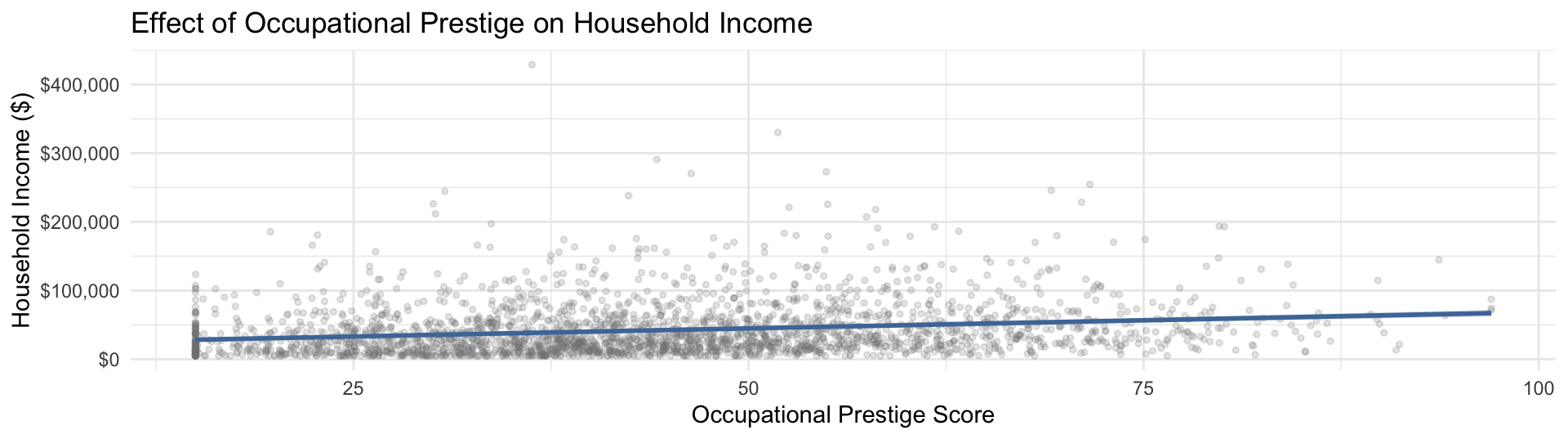
Use geom_smooth(method = "lm") to overlay the regression line on a scatterplot:

ggplot(attain_reg, aes(x = prestg80, y = income91)) +
  geom_point(alpha = 0.2, color = "gray50", size = 1) +
  geom_smooth(method = "lm", se = TRUE,
              color = "#4E79A7", fill = "#4E79A7", alpha = 0.2) +
  scale_y_continuous(labels = scales::dollar_format()) +
  labs(title = "Effect of Occupational Prestige on Household Income",
       x = "Occupational Prestige Score", y = "Household Income ($)") +
  theme_minimal(base_size = 11)

modelplot() from modelsummary shows coefficients with 95% confidence intervals. If the CI does not cross 0, the coefficient is significant at \(\alpha = 0.05\):

modelplot(model_biv, coef_omit = "Intercept") +
  geom_vline(xintercept = 0, linetype = "dashed", color = "#E15759") +
  labs(title = "OLS Coefficient: Effect of Prestige on Income",
       x = "Estimated Coefficient ($ per prestige point)") +
  theme_minimal(base_size = 11)

Questions?

Part 3: Regression with Categorical Predictors

When your key predictor has categories

Categorical Variables: The Challenge

So far our key predictor has been continuous (occupational prestige). What if the key predictor is categorical — like educational degree, sex, or race?

The challenge: We can’t multiply a category label by a number. Regression needs numbers.

The solution: Replace a categorical variable with a set of dummy (indicator) variables — one for each category except the baseline.

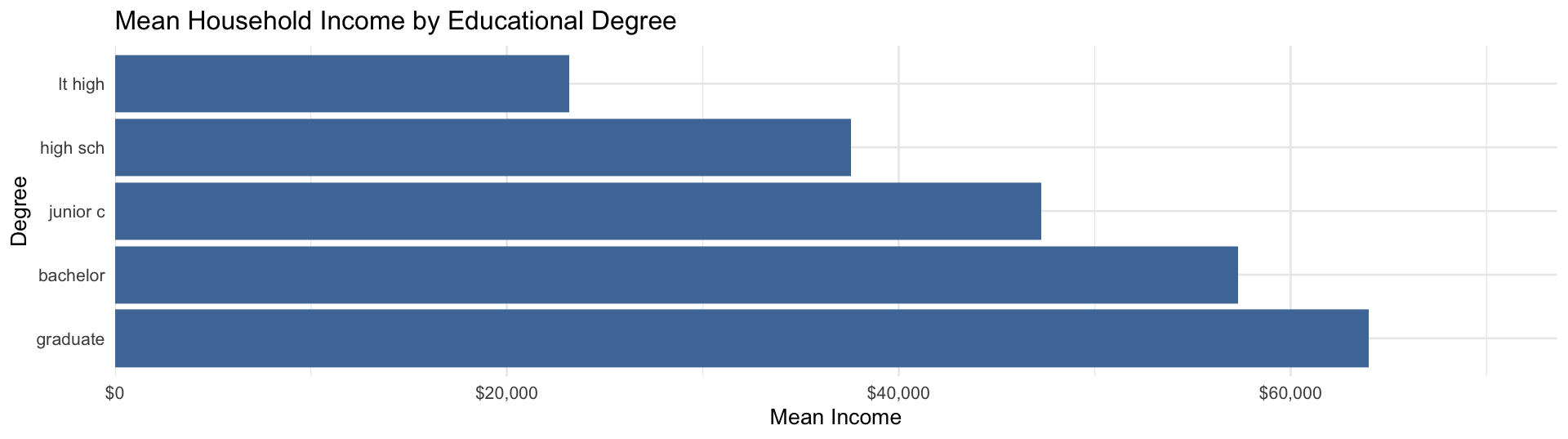
We can see groups differ — but how much? And is the difference significant? Regression tells us.

Dummy Variables and Baseline Categories

For a categorical variable with k categories, we create k − 1 dummy variables. The omitted category is the baseline (reference) group — all comparisons are made against it.

Example: Degree (5 categories) → 4 dummies (baseline = lt high [less than high school]):

Degree Dummy variable R creates Predicted income
lt high (baseline) (omitted — absorbed into intercept) \(\alpha\)
High School degree_fhigh sch = 1, all others = 0 \(\alpha + b_1\)
Junior College degree_fjunior c = 1, all others = 0 \(\alpha + b_2\)
Bachelor’s degree_fbachelor = 1, all others = 0 \(\alpha + b_3\)
Graduate degree_fgraduate = 1, all others = 0 \(\alpha + b_4\)

Each coefficient (\(b_1, b_2, \ldots\)) = predicted income above or below the baseline group.

The baseline’s predicted income = the intercept α. Every other coefficient = income above or below that baseline.

Choosing the baseline:

  • Pick the category that makes theoretical sense as a reference point
  • Common choices: lowest category, largest group, or the “control” condition
  • In R: fct_relevel(var, "category_name") (from forcats, loaded with tidyverse)

Setting Up Categorical IVs in R

Before setting a baseline, see what categories exist:

# What categories does degree have?
table(attain$degree)

bachelor graduate high sch junior c  lt high 
     497      216     1586      176      507 

The first value alphabetically becomes the default baseline — we usually want to choose explicitly.

attain_cat <- attain |>
  filter(!is.na(degree), !is.na(income91)) |>
  mutate(
    # Specify all levels in educational order (lowest → highest)
    degree_f = fct_relevel(degree, "lt high", "high sch", "junior c", "bachelor", "graduate")
  )

# Verify: levels listed in educational order, first = baseline
levels(attain_cat$degree_f)
[1] "lt high"  "high sch" "junior c" "bachelor" "graduate"

Choosing the baseline category:

  • Always choose a category that makes theoretical sense as a reference point
  • Common strategy: use the group that represents “no treatment” or the lowest level — e.g., less than high school when testing whether higher degrees predict income
  • Avoid making the smallest group the baseline — comparisons to a tiny group are imprecise
  • Example: if your hypothesis is about the disadvantage of not having a college degree, set "bachelor" as the baseline so coefficients show penalty for each lower degree level

Baseline in our example:

"lt high" (less than high school) is the baseline. Every other coefficient shows how much more income people with that degree earn compared to respondents without a high school diploma.

model_cat <- lm(income91 ~ degree_f, data = attain_cat)

modelsummary(model_cat,
             coef_rename = c("(Intercept)"        = "Intercept",
                             "degree_fhigh sch"   = "High School",
                             "degree_fjunior c"   = "Junior College",
                             "degree_fbachelor"   = "Bachelor's Degree",
                             "degree_fgraduate"   = "Graduate Degree"),
             stars   = TRUE,
             title   = "OLS: Income ~ Degree (baseline = lt high)",
             gof_map = c("nobs", "r.squared"))
OLS: Income ~ Degree (baseline = lt high)
 (1)
Intercept 23181.028***
(1765.437)
High School 14360.115***
(2014.784)
Junior College 24106.743***
(3357.712)
Bachelor's Degree 34134.344***
(2459.053)
Graduate Degree 40821.525***
(3156.575)
Num.Obs. 2632
R2 0.099
+ p < 0.1, * p < 0.05, ** p < 0.01, *** p < 0.001

Interpreting Categorical Coefficients

With degree as the key predictor (baseline = lt high [less than HS]):

\[\widehat{\text{income}} = \alpha + b_{\text{hs}} X_{\text{hs}} + b_{\text{jc}} X_{\text{jc}} + b_{\text{ba}} X_{\text{ba}} + b_{\text{grad}} X_{\text{grad}}\]

Each \(X\) is a dummy variable (0/1) for that degree level; each coefficient = the income difference relative to the baseline group.

Reading categorical coefficients:

Intercept (\(\alpha\)): Predicted income for someone with less than a high school degree (the baseline). This is interpretable — it’s the baseline group’s average income.

Coefficient on High School (\(b_{\text{hs}}\)): On average, having a high school diploma (vs. less than HS) is associated with $X more in household income.

Coefficient on Graduate Degree (\(b_{\text{grad}}\)): On average, having a graduate degree (vs. less than HS) is associated with $Y more in household income.

Key insight: Regression with a categorical IV is equivalent to comparing group means — but regression gives us p-values for each comparison and allows us to control for other variables.

# Predicted income for each degree level — ordered lowest to highest
tibble(
  Degree   = c("Less than HS (baseline)", "High School", "Junior College",
               "Bachelor's Degree", "Graduate Degree"),
  degree_f = factor(
    c("lt high", "high sch", "junior c", "bachelor", "graduate"),
    levels = levels(attain_cat$degree_f)
  )
) |>
  mutate(Predicted_Income = scales::dollar(
    round(predict(model_cat, newdata = pick(degree_f)), 0)
  )) |>
  select(Degree, Predicted_Income)
# A tibble: 5 × 2
  Degree                  Predicted_Income
  <chr>                   <chr>           
1 Less than HS (baseline) $23,181         
2 High School             $37,541         
3 Junior College          $47,288         
4 Bachelor's Degree       $57,315         
5 Graduate Degree         $64,003         
# Rename and reverse order so lowest degree appears at top (matching table above)
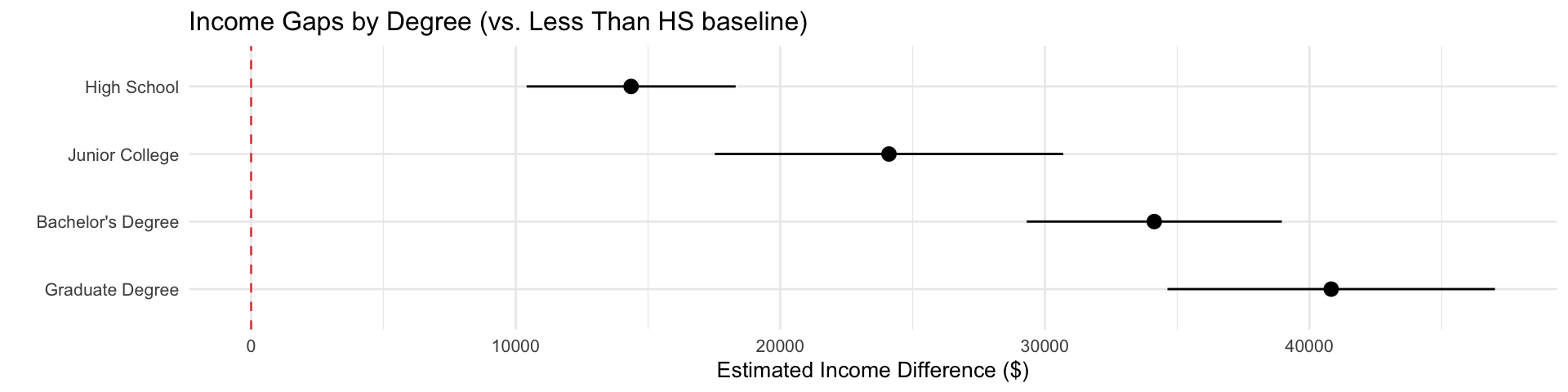
modelplot(
  model_cat,
  coef_omit = "Intercept",
  coef_rename = c(
    "degree_fhigh sch" = "High School",
    "degree_fjunior c" = "Junior College",
    "degree_fbachelor" = "Bachelor's Degree",
    "degree_fgraduate" = "Graduate Degree"
  )
) +
  scale_y_discrete(limits = rev) +   # lowest degree (HS) at top
  geom_vline(xintercept = 0, linetype = "dashed", color = "#E15759") +
  labs(
    title = "Income Gaps by Degree (vs. Less Than HS baseline)",
    x = "Estimated Income Difference ($)"
  ) +
  theme_minimal(base_size = 10)

Questions?

Part 4: OLS Assumptions

When can we trust our estimates?

The Four OLS Assumptions

Observations are independent — typically satisfied by random sampling.

  • Violated when observations are clustered (e.g., students within schools)
  • Fix: include survey weights or use clustered standard errors
# If your data have survey weights:
lm(outcome ~ predictor, data = data, weights = wt_var)

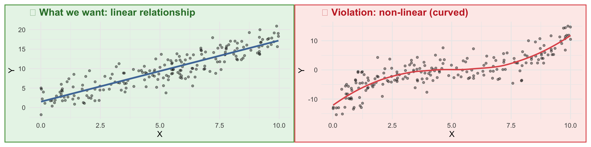
There is a linear relationship between the continuous IV and the outcome.

Always check this with a scatter plot of Y vs X before running the regression.

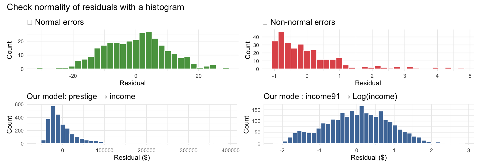
The errors are approximately normally distributed — most important in small samples. In large samples, violations are usually not a big problem (Central Limit Theorem applies).

What we did in this class:

The raw income91 variable is right-skewed (common with income data), which produces non-normal residuals in the bottom-left panel. Running log(income91) as the outcome — model_log above — produces the more symmetric residuals in the bottom-right panel. This is a standard fix: when your outcome is right-skewed, log-transforming it often corrects the non-normality of errors.

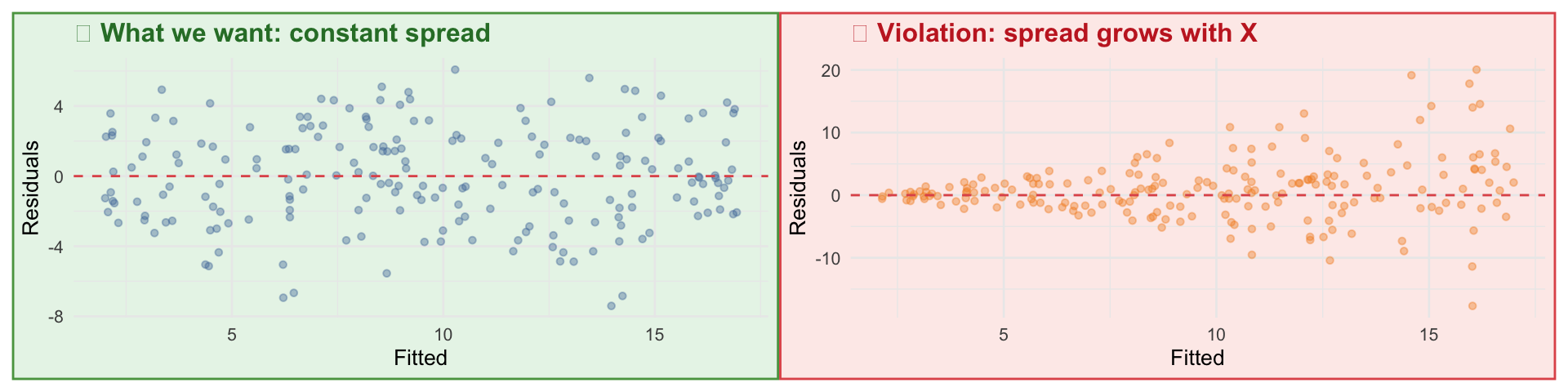
The spread of residuals is constant across all values of X (equal variance).

Violations bias standard errors — important for t-tests. Fix: robust standard errors.

Checking Assumptions Visually

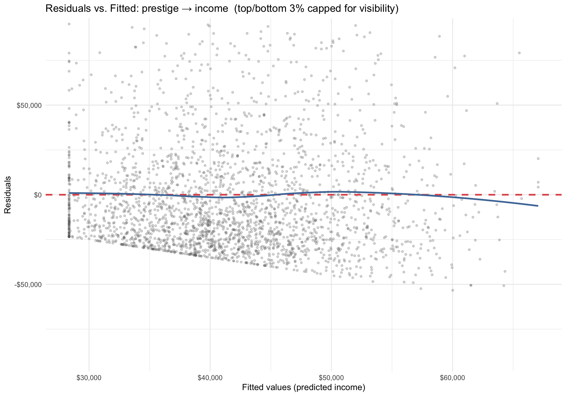
A residuals vs. fitted plot diagnoses both linearity and homoskedasticity at once:

What to look for — and what our model shows:

Linearity: Is the blue loess line approximately flat (horizontal)? In our model: mostly flat with slight curvature — no major concern.

Homoskedasticity: Is the vertical spread of points roughly constant across the x-axis? In our model: the spread is roughly similar across fitted values, though slightly wider at high incomes — common with income data.

Overall, our prestige → income model does not show dramatic assumption violations, but some heteroskedasticity is plausible. Using vcov = "HC1" robust SEs (shown next) is a most common precaution used.

Robust Standard Errors

If you suspect heteroskedasticity, use robust standard errors — they correct the SEs without changing the coefficient estimates:

  • Violations of normality and homoskedasticity do not bias coefficient estimates (\(a\), \(b\))
  • But they do bias the standard errors — which affects t-statistics and p-values
  • Robust SEs account for these violations with a conservative adjustment

The easiest approach is to compare standard vs. robust SEs side-by-side using modelsummary():

modelsummary(
  list("Standard SEs" = model_biv, "Robust (HC1) SEs" = model_biv),
  vcov = list("classical", "HC1"),
  coef_rename = c("(Intercept)" = "Intercept",
                  "prestg80"    = "Prestige Score"),
  stars = TRUE,
  gof_map = c("nobs", "r.squared"),
  title = "Standard vs. Robust Standard Errors"
)
Standard vs. Robust Standard Errors
Standard SEs Robust (HC1) SEs
Intercept 21273.309*** 21273.309***
(2134.090) (1947.377)
Prestige Score 472.133*** 472.133***
(45.943) (44.781)
Num.Obs. 2527 2527
R2 0.040 0.040
+ p < 0.1, * p < 0.05, ** p < 0.01, *** p < 0.001

What Do Control Variables Do?

When we add a control variable to a regression, we are partitioning the variation in the outcome:

Without a control:

\[\text{income} = a + b_1{\text{prestige}} + e\]

The coefficient \(b_1\) captures all the ways prestige is associated with income — including variation that is really due to sex (because men and women differ in both prestige and income).

With a control for sex:

\[\text{income} = a + b_1\text{prestige} + b_2\text{sex} + e\]

Now \(b_1\) captures the association between prestige and income after filtering out any variation that could be due to sex differences. We are comparing people who are identical on the control variable (same sex) and asking: does prestige still predict income?

The key intuition:

A control variable “filters away” variation in the outcome that is explained by that control. The coefficient on the key predictor then reflects only the variation that can’t be explained by the control variables. This is what “holding constant” means statistically.

Multiple Regression

We can include multiple predictors — this is multiple regression. We’ll cover this in depth in Week 13.

attain_multi <- attain |>
  filter(!is.na(prestg80), !is.na(income91), !is.na(sex)) |>
  mutate(sex_f = fct_relevel(sex, "male"))

model_biv2   <- lm(income91 ~ prestg80,          data = attain_multi)
model_multi  <- lm(income91 ~ prestg80 + sex_f,   data = attain_multi)
modelsummary(
  list("Bivariate" = model_biv2, "Multiple" = model_multi),
  coef_rename = c("(Intercept)" = "Intercept",
                  "prestg80"    = "Prestige Score",
                  "sex_ffemale" = "Female"),
  stars   = TRUE,
  title   = "Prestige and Income: Bivariate vs. Multiple",
  gof_map = c("nobs", "r.squared")
)
Prestige and Income: Bivariate vs. Multiple
Bivariate Multiple
Intercept 21273.309*** 23949.643***
(2134.090) (2295.876)
Prestige Score 472.133*** 469.766***
(45.943) (45.869)
Female −4702.028**
(1503.645)
Num.Obs. 2527 2527
R2 0.040 0.044
+ p < 0.1, * p < 0.05, ** p < 0.01, *** p < 0.001

Reading the multiple regression table:

Coefficient on Prestige Score (bivariate → multiple): $472 → $470 per prestige point. After controlling for sex, the prestige slope changes slightly — this shift tells us how much of the bivariate prestige effect was actually due to sex differences in prestige.

Coefficient on Female: $-4702 — women earn about $4702 less per year than men at the same prestige level. This is the gender income gap net of occupational status.

R² increase: 4% (bivariate) → 4.4% (multiple regression). Adding sex explains additional variation in income beyond prestige alone — but most variation in income remains unexplained by these two predictors.

In Week 13, we’ll cover how to decide which controls to include, and what changes in coefficients across models mean theoretically.

Reading Research: Thompson & Keith (2001)

Seeing today’s tools published in a classical sociological study

“The Blacker the Berry” — Overview

Thompson, M.S. & Keith, V.M. (2001). The Blacker the Berry: Gender, Skin Tone, Self-Esteem, and Self-Efficacy. Gender & Society, 15(3), 336–357.

Research question: Does skin tone predict psychological well-being — specifically self-esteem and self-efficacy — for Black Americans? And does this relationship differ by gender?

  • Motivated by colorism: the documented pattern in which lighter-skinned Black individuals receive preferential treatment in U.S. society
  • “The blacker the berry, the sweeter the juice” is a common idiom that celebrates dark skin tones in Black individuals — serving as a counter-narrative to colorism. The authors ask whether this affirmation holds for Black Americans’ own self-perception

Why this paper?

This is a model of how to use OLS regression to answer a sociological question. The authors carefully choose their outcome variable, identify a clear key predictor, include theoretically motivated controls, and interpret the substantive meaning of their coefficients.

Research Design

  • Data: National Survey of Black Americans (NSBA), 1979–1980
  • Sample: 2,107 Black American adults; analyses conducted separately for men (n ≈ 581) and women (n ≈ 1,035) who are employed
  • Why separate models? The authors hypothesize that the relationship between skin tone and self-esteem differs by gender. Running separate regressions for men and women is similar in spirit to including an interaction term (which we’ll cover in Week 13), but the authors chose this approach for simplicity — because they test multiple interactions across several controls, splitting the sample is more tractable than modeling every interaction explicitly
Role Variable Measurement
Outcome (DV) 1 Self-esteem Rosenberg 10-item scale (1–4; higher = more positive)
Outcome (DV) 2 Self-efficacy Personal efficacy scale (1–4; higher = more control)
Key predictor Skin tone Interviewer-rated 5-point scale: 1 = very dark to 5 = very light brown
Controls Education, income, employment, age, marital status, family origin Standard socioeconomic controls

Self-esteem vs. self-efficacy — what’s the difference?

Self-esteem is a person’s overall sense of their own value or worth — “Do I feel good about myself?” It reflects how positively someone regards themselves as a person.

Self-efficacy is a person’s belief in their ability to control outcomes in their own life — “Can I make things happen?” It reflects how much agency or personal power someone feels they have.

These are related but distinct psychological constructs. The authors study both because colorism may affect not just how you feel about yourself (self-esteem) but also your sense of whether your efforts can shape your future (self-efficacy).

The authors estimate (separately for men and women):

\[\widehat{\text{self-esteem}} = \alpha + \beta_1\text{skin tone} + \beta_2\text{educ} + \beta_3\text{income} + \cdots + e\]

Connecting to today:

  • Outcome variable: self-esteem or self-efficacy (continuous DV)
  • Key predictor: skin tone (treated as continuous — 5-point scale)
  • Controls: education, income, age, etc. — “filtered away” so the skin tone coefficient reflects prestige net of SES differences

Key Results

Simplified version of Tables 2 & 3 from Thompson & Keith (2001). Skin tone scale: 1 = very dark, 5 = very light — a higher score means lighter skin, so a positive coefficient indicates lighter skin → higher outcome.

Women Men
Variable Self-Esteem Self-Efficacy Self-Esteem Self-Efficacy
Skin tone .187* .029 .088 .208†
Education .053† .127*** .036 .126***
Income .025 .054*** .019 .014
Age .034*** .033*** .019** .030***
Employed .292 −.093 .449† −.378
N 1,036 1,036 647 647
.092 .096 .072 .093

†p ≤ .10. p ≤ .05. p ≤ .01. p ≤ .001. Coefficients are unstandardized OLS estimates from fully adjusted models (Model 4). Adapted from Thompson & Keith (2001), Tables 2 & 3.

The key result:

Lighter skin tone (higher score) significantly predicts higher self-esteem for Black women (.187*), but not for men, and not for self-efficacy once SES is controlled — colorism operates through gender and is outcome-specific.

The skin tone coefficient tells a split story across the two outcomes:

  • Self-esteem: coefficient = .187* (\(p < 0.05\)) — lighter skin (higher score) → higher self-esteem. A Black woman rated 4 (lighter) is predicted to have meaningfully higher self-esteem than a Black woman rated 2 (darker), even after controlling for education, income, and other SES factors
  • Self-efficacy: coefficient = .029 (not significant) — once SES is controlled, skin tone does not significantly predict self-efficacy for women

Interpretation: Colorism shapes how Black women feel about their worth (self-esteem) but not their sense of personal agency (self-efficacy) in the fully adjusted model.

The skin tone coefficients are weaker and largely non-significant for men:

  • Self-esteem: coefficient = .088 (not significant) — skin tone does not predict self-esteem for Black men
  • Self-efficacy: coefficient = .208† (\(p ≤ .10\), borderline) — a marginal suggestion that lighter skin is associated with higher self-efficacy, but this falls short of conventional significance

Why the difference? The authors argue that beauty ideals — which prize lighter skin — operate much more strongly as a social evaluation system for women than for men. For men, occupational and economic status matter more than appearance-based judgments.

Colorism operates through gender — and is outcome-specific:

For Black women, lighter skin predicts higher self-esteem (.187*) even after controlling for SES — but skin tone does not significantly predict self-efficacy. For Black men, skin tone has no significant effect on self-esteem, and only a marginal effect on self-efficacy (.208†). This finding demonstrates that colorism is not just about race — it is deeply shaped by gender, and its psychological effects depend on which dimension of self-evaluation we examine.

The magnitude matters here: the authors don’t just report that the relationship is significant — they discuss whether the coefficient size is large enough to be practically meaningful. This is exactly the “statistical vs. substantive significance” distinction we covered today.

Connecting Thompson & Keith to Today

Today’s concept In Thompson & Keith
Outcome variable Self-esteem, self-efficacy
Key predictor Skin tone (the main theoretical variable)
Control variables Education, income, age — “filtered away”
OLS regression lm(selfesteem ~ skintone + educ + income + ...)
Coefficient interpretation Each skin tone point → X-unit change in self-esteem
Statistical vs. substantive significance Is the effect real AND meaningful?
Separate models by group Week 13 — interaction terms capture this more formally

For your research paper:

Thompson & Keith is a model for how to write up regression results in a paper. Notice: they state the research question clearly, justify their variable choices, report coefficients with standard errors, discuss magnitude, and connect the statistical results back to the sociological theory.

Questions?

Key Takeaways

  • The outcome variable (Y) is what you are trying to explain — also called the dependent variable
  • The key predictor (X) is the main theoretical variable — also called the key independent variable
  • OLS estimates the slope (\(b\)): average change in outcome per one-unit increase in the predictor
  • OLS minimizes the sum of squared residuals — that’s where “least squares” comes from
  • Every coefficient has its own t-test: \(t = b / SE(b)\), same logic as Week 9
  • is the proportion of variation in Y explained by the model — always report and interpret it

Connection to Week 9:

Each regression coefficient has its own null hypothesis (\(H_0: \beta = 0\)) and its own t-test and p-value. The inference logic from Week 9 applies directly — the only thing new is the shape of the model.

  • Use fct_relevel(var, "baseline") to set the comparison group
  • Each dummy variable coefficient = difference from the baseline in the outcome variable
  • The intercept = predicted outcome for the baseline group (interpretable!)
  • Always state your baseline category when reporting results
Assumption How to check Fix if violated
Independence Study design Survey weights, clustered SEs
Linearity Scatter plot Y vs X Transform variables (e.g., log)
Normal errors Histogram of residuals Usually OK in large samples
Homoskedasticity Residuals vs. fitted plot Robust standard errors (vcov = "HC1")

Why This Matters for Your Research Paper

  • HW #9 asks you to run an OLS regression on your research data — today’s tools are exactly what you need
  • Your revised proposal (due 4/16) should now describe which regression model you plan to use
  • Your final paper will likely use OLS regression as its central analysis

What HW #9 asks — and what you now know how to do:

  1. Identify your outcome and key predictor → Part 1 today
  2. Run lm() and display results with modelsummary() → Part 2 today
  3. Set a baseline if using a categorical predictor → Part 3 today
  4. Interpret the coefficient magnitude, p-value, and R² → Part 2 today
  5. Visualize the relationship with a scatter + regression line (continuous IV) or coefficient plot → Part 2 today

One thing to add to your thinking for hw9:

When interpreting your results, distinguish statistical significance (is \(p < 0.05\)?) from substantive significance (does the size of the coefficient actually matter in the real world?). Both belong in your write-up.

Questions?

Assignments

Weekly Assignment #9Due Thursday, April 9

Using your research dataset:

  1. State a research question with a continuous outcome variable and at least one key predictor
  2. Write your hypothesis (direction of expected relationship and justification)
  3. Run OLS regression with lm() and display results with modelsummary()
  4. If using a categorical predictor: use fct_relevel(var, "baseline_category") to set a baseline, and state what it is
  5. Interpret the estimated coefficient(s): direction, magnitude, and what they mean
  6. Report and interpret
  7. Visualize: scatter plot with regression line (continuous IV) or coefficient plot
  8. Discuss both statistical and substantive significance

Also due:

  • HW #8Due Thursday, April 2 (hypothesis testing)
  • Revised Proposal with OutlineDue Thursday, April 16

In-class lab today:

  • Practice running OLS on your own dataset and interpreting the output